Design and Analysis of Algorithms Lab Manual Using Java
Design and Analysis Quick Guide
Design and Analysis Introduction
An algorithm is a set of steps of operations to solve a problem performing calculation, data processing, and automated reasoning tasks. An algorithm is an efficient method that can be expressed within finite amount of time and space.
An algorithm is the best way to represent the solution of a particular problem in a very simple and efficient way. If we have an algorithm for a specific problem, then we can implement it in any programming language, meaning that the algorithm is independent from any programming languages.
Algorithm Design
The important aspects of algorithm design include creating an efficient algorithm to solve a problem in an efficient way using minimum time and space.
To solve a problem, different approaches can be followed. Some of them can be efficient with respect to time consumption, whereas other approaches may be memory efficient. However, one has to keep in mind that both time consumption and memory usage cannot be optimized simultaneously. If we require an algorithm to run in lesser time, we have to invest in more memory and if we require an algorithm to run with lesser memory, we need to have more time.
Problem Development Steps
The following steps are involved in solving computational problems.
- Problem definition
- Development of a model
- Specification of an Algorithm
- Designing an Algorithm
- Checking the correctness of an Algorithm
- Analysis of an Algorithm
- Implementation of an Algorithm
- Program testing
- Documentation
Characteristics of Algorithms
The main characteristics of algorithms are as follows −
-
Algorithms must have a unique name
-
Algorithms should have explicitly defined set of inputs and outputs
-
Algorithms are well-ordered with unambiguous operations
-
Algorithms halt in a finite amount of time. Algorithms should not run for infinity, i.e., an algorithm must end at some point
Pseudocode
Pseudocode gives a high-level description of an algorithm without the ambiguity associated with plain text but also without the need to know the syntax of a particular programming language.
The running time can be estimated in a more general manner by using Pseudocode to represent the algorithm as a set of fundamental operations which can then be counted.
Difference between Algorithm and Pseudocode
An algorithm is a formal definition with some specific characteristics that describes a process, which could be executed by a Turing-complete computer machine to perform a specific task. Generally, the word "algorithm" can be used to describe any high level task in computer science.
On the other hand, pseudocode is an informal and (often rudimentary) human readable description of an algorithm leaving many granular details of it. Writing a pseudocode has no restriction of styles and its only objective is to describe the high level steps of algorithm in a much realistic manner in natural language.
For example, following is an algorithm for Insertion Sort.
Algorithm: Insertion-Sort Input: A list L of integers of length n Output: A sorted list L1 containing those integers present in L Step 1: Keep a sorted list L1 which starts off empty Step 2: Perform Step 3 for each element in the original list L Step 3: Insert it into the correct position in the sorted list L1. Step 4: Return the sorted list Step 5: Stop
Here is a pseudocode which describes how the high level abstract process mentioned above in the algorithm Insertion-Sort could be described in a more realistic way.
for i <- 1 to length(A) x <- A[i] j <- i while j > 0 and A[j-1] > x A[j] <- A[j-1] j <- j - 1 A[j] <- x
In this tutorial, algorithms will be presented in the form of pseudocode, that is similar in many respects to C, C++, Java, Python, and other programming languages.
Design and Analysis of Algorithm
In theoretical analysis of algorithms, it is common to estimate their complexity in the asymptotic sense, i.e., to estimate the complexity function for arbitrarily large input. The term "analysis of algorithms" was coined by Donald Knuth.
Algorithm analysis is an important part of computational complexity theory, which provides theoretical estimation for the required resources of an algorithm to solve a specific computational problem. Most algorithms are designed to work with inputs of arbitrary length. Analysis of algorithms is the determination of the amount of time and space resources required to execute it.
Usually, the efficiency or running time of an algorithm is stated as a function relating the input length to the number of steps, known as time complexity, or volume of memory, known as space complexity.
The Need for Analysis
In this chapter, we will discuss the need for analysis of algorithms and how to choose a better algorithm for a particular problem as one computational problem can be solved by different algorithms.
By considering an algorithm for a specific problem, we can begin to develop pattern recognition so that similar types of problems can be solved by the help of this algorithm.
Algorithms are often quite different from one another, though the objective of these algorithms are the same. For example, we know that a set of numbers can be sorted using different algorithms. Number of comparisons performed by one algorithm may vary with others for the same input. Hence, time complexity of those algorithms may differ. At the same time, we need to calculate the memory space required by each algorithm.
Analysis of algorithm is the process of analyzing the problem-solving capability of the algorithm in terms of the time and size required (the size of memory for storage while implementation). However, the main concern of analysis of algorithms is the required time or performance. Generally, we perform the following types of analysis −
-
Worst-case − The maximum number of steps taken on any instance of size a.
-
Best-case − The minimum number of steps taken on any instance of size a.
-
Average case − An average number of steps taken on any instance of size a.
-
Amortized − A sequence of operations applied to the input of size a averaged over time.
To solve a problem, we need to consider time as well as space complexity as the program may run on a system where memory is limited but adequate space is available or may be vice-versa. In this context, if we compare bubble sort and merge sort. Bubble sort does not require additional memory, but merge sort requires additional space. Though time complexity of bubble sort is higher compared to merge sort, we may need to apply bubble sort if the program needs to run in an environment, where memory is very limited.
Design and Analysis Methodology
To measure resource consumption of an algorithm, different strategies are used as discussed in this chapter.
Asymptotic Analysis
The asymptotic behavior of a function f(n) refers to the growth of f(n) as n gets large.
We typically ignore small values of n, since we are usually interested in estimating how slow the program will be on large inputs.
A good rule of thumb is that the slower the asymptotic growth rate, the better the algorithm. Though it's not always true.
For example, a linear algorithm $f(n) = d * n + k$ is always asymptotically better than a quadratic one, $f(n) = c.n^2 + q$.
Solving Recurrence Equations
A recurrence is an equation or inequality that describes a function in terms of its value on smaller inputs. Recurrences are generally used in divide-and-conquer paradigm.
Let us consider T(n) to be the running time on a problem of size n.
If the problem size is small enough, say n < c where c is a constant, the straightforward solution takes constant time, which is written as θ(1). If the division of the problem yields a number of sub-problems with size $\frac{n}{b}$.
To solve the problem, the required time is a.T(n/b) . If we consider the time required for division is D(n) and the time required for combining the results of sub-problems is C(n) , the recurrence relation can be represented as −
$$T(n)=\begin{cases}\:\:\:\:\:\:\:\:\:\:\:\:\:\:\:\:\:\:\:\:\:\:\:\theta(1) & if\:n\leqslant c\\a T(\frac{n}{b})+D(n)+C(n) & otherwise\end{cases}$$
A recurrence relation can be solved using the following methods −
-
Substitution Method − In this method, we guess a bound and using mathematical induction we prove that our assumption was correct.
-
Recursion Tree Method − In this method, a recurrence tree is formed where each node represents the cost.
-
Master's Theorem − This is another important technique to find the complexity of a recurrence relation.
Amortized Analysis
Amortized analysis is generally used for certain algorithms where a sequence of similar operations are performed.
-
Amortized analysis provides a bound on the actual cost of the entire sequence, instead of bounding the cost of sequence of operations separately.
-
Amortized analysis differs from average-case analysis; probability is not involved in amortized analysis. Amortized analysis guarantees the average performance of each operation in the worst case.
It is not just a tool for analysis, it's a way of thinking about the design, since designing and analysis are closely related.
Aggregate Method
The aggregate method gives a global view of a problem. In this method, if n operations takes worst-case time T(n) in total. Then the amortized cost of each operation is T(n)/n . Though different operations may take different time, in this method varying cost is neglected.
Accounting Method
In this method, different charges are assigned to different operations according to their actual cost. If the amortized cost of an operation exceeds its actual cost, the difference is assigned to the object as credit. This credit helps to pay for later operations for which the amortized cost less than actual cost.
If the actual cost and the amortized cost of ith operation are $c_{i}$ and $\hat{c_{l}}$, then
$$\displaystyle\sum\limits_{i=1}^n \hat{c_{l}}\geqslant\displaystyle\sum\limits_{i=1}^n c_{i}$$
Potential Method
This method represents the prepaid work as potential energy, instead of considering prepaid work as credit. This energy can be released to pay for future operations.
If we perform n operations starting with an initial data structure D0 . Let us consider, ci as the actual cost and Di as data structure of ith operation. The potential function Ф maps to a real number Ф( Di ), the associated potential of Di . The amortized cost $\hat{c_{l}}$ can be defined by
$$\hat{c_{l}}=c_{i}+\Phi (D_{i})-\Phi (D_{i-1})$$
Hence, the total amortized cost is
$$\displaystyle\sum\limits_{i=1}^n \hat{c_{l}}=\displaystyle\sum\limits_{i=1}^n (c_{i}+\Phi (D_{i})-\Phi (D_{i-1}))=\displaystyle\sum\limits_{i=1}^n c_{i}+\Phi (D_{n})-\Phi (D_{0})$$
Dynamic Table
If the allocated space for the table is not enough, we must copy the table into larger size table. Similarly, if large number of members are erased from the table, it is a good idea to reallocate the table with a smaller size.
Using amortized analysis, we can show that the amortized cost of insertion and deletion is constant and unused space in a dynamic table never exceeds a constant fraction of the total space.
In the next chapter of this tutorial, we will discuss Asymptotic Notations in brief.
Asymptotic Notations and Apriori Analysis
In designing of Algorithm, complexity analysis of an algorithm is an essential aspect. Mainly, algorithmic complexity is concerned about its performance, how fast or slow it works.
The complexity of an algorithm describes the efficiency of the algorithm in terms of the amount of the memory required to process the data and the processing time.
Complexity of an algorithm is analyzed in two perspectives: Time and Space.
Time Complexity
It's a function describing the amount of time required to run an algorithm in terms of the size of the input. "Time" can mean the number of memory accesses performed, the number of comparisons between integers, the number of times some inner loop is executed, or some other natural unit related to the amount of real time the algorithm will take.
Space Complexity
It's a function describing the amount of memory an algorithm takes in terms of the size of input to the algorithm. We often speak of "extra" memory needed, not counting the memory needed to store the input itself. Again, we use natural (but fixed-length) units to measure this.
Space complexity is sometimes ignored because the space used is minimal and/or obvious, however sometimes it becomes as important an issue as time.
Asymptotic Notations
Execution time of an algorithm depends on the instruction set, processor speed, disk I/O speed, etc. Hence, we estimate the efficiency of an algorithm asymptotically.
Time function of an algorithm is represented by T(n), where n is the input size.
Different types of asymptotic notations are used to represent the complexity of an algorithm. Following asymptotic notations are used to calculate the running time complexity of an algorithm.
-
O − Big Oh
-
Ω − Big omega
-
θ − Big theta
-
o − Little Oh
-
ω − Little omega
O: Asymptotic Upper Bound
'O' (Big Oh) is the most commonly used notation. A function f(n) can be represented is the order of g(n) that is O(g(n)) , if there exists a value of positive integer n as n0 and a positive constant c such that −
$f(n)\leqslant c.g(n)$ for $n > n_{0}$ in all case
Hence, function g(n) is an upper bound for function f(n) , as g(n) grows faster than f(n) .
Example
Let us consider a given function, $f(n) = 4.n^3 + 10.n^2 + 5.n + 1$
Considering $g(n) = n^3$,
$f(n)\leqslant 5.g(n)$ for all the values of $n > 2$
Hence, the complexity of f(n) can be represented as $O(g(n))$, i.e. $O(n^3)$
Ω: Asymptotic Lower Bound
We say that $f(n) = \Omega (g(n))$ when there exists constant c that $f(n)\geqslant c.g(n)$ for all sufficiently large value of n. Here n is a positive integer. It means function g is a lower bound for function f ; after a certain value of n, f will never go below g .
Example
Let us consider a given function, $f(n) = 4.n^3 + 10.n^2 + 5.n + 1$.
Considering $g(n) = n^3$, $f(n)\geqslant 4.g(n)$ for all the values of $n > 0$.
Hence, the complexity of f(n) can be represented as $\Omega (g(n))$, i.e. $\Omega (n^3)$
θ: Asymptotic Tight Bound
We say that $f(n) = \theta(g(n))$ when there exist constants c1 and c2 that $c_{1}.g(n) \leqslant f(n) \leqslant c_{2}.g(n)$ for all sufficiently large value of n. Here n is a positive integer.
This means function g is a tight bound for function f.
Example
Let us consider a given function, $f(n) = 4.n^3 + 10.n^2 + 5.n + 1$
Considering $g(n) = n^3$, $4.g(n) \leqslant f(n) \leqslant 5.g(n)$ for all the large values of n.
Hence, the complexity of f(n) can be represented as $\theta (g(n))$, i.e. $\theta (n^3)$.
O - Notation
The asymptotic upper bound provided by O-notation may or may not be asymptotically tight. The bound $2.n^2 = O(n^2)$ is asymptotically tight, but the bound $2.n = O(n^2)$ is not.
We use o-notation to denote an upper bound that is not asymptotically tight.
We formally define o(g(n)) (little-oh of g of n) as the set f(n) = o(g(n)) for any positive constant $c > 0$ and there exists a value $n_{0} > 0$, such that $0 \leqslant f(n) \leqslant c.g(n)$.
Intuitively, in the o-notation, the function f(n) becomes insignificant relative to g(n) as n approaches infinity; that is,
$$\lim_{n \rightarrow \infty}\left(\frac{f(n)}{g(n)}\right) = 0$$
Example
Let us consider the same function, $f(n) = 4.n^3 + 10.n^2 + 5.n + 1$
Considering $g(n) = n^{4}$,
$$\lim_{n \rightarrow \infty}\left(\frac{4.n^3 + 10.n^2 + 5.n + 1}{n^4}\right) = 0$$
Hence, the complexity of f(n) can be represented as $o(g(n))$, i.e. $o(n^4)$.
ω – Notation
We use ω-notation to denote a lower bound that is not asymptotically tight. Formally, however, we define ω(g(n)) (little-omega of g of n) as the set f(n) = ω(g(n)) for any positive constant C > 0 and there exists a value $n_{0} > 0$, such that $0 \leqslant c.g(n) < f(n)$.
For example, $\frac{n^2}{2} = \omega (n)$, but $\frac{n^2}{2} \neq \omega (n^2)$. The relation $f(n) = \omega (g(n))$ implies that the following limit exists
$$\lim_{n \rightarrow \infty}\left(\frac{f(n)}{g(n)}\right) = \infty$$
That is, f(n) becomes arbitrarily large relative to g(n) as n approaches infinity.
Example
Let us consider same function, $f(n) = 4.n^3 + 10.n^2 + 5.n + 1$
Considering $g(n) = n^2$,
$$\lim_{n \rightarrow \infty}\left(\frac{4.n^3 + 10.n^2 + 5.n + 1}{n^2}\right) = \infty$$
Hence, the complexity of f(n) can be represented as $o(g(n))$, i.e. $\omega (n^2)$.
Apriori and Apostiari Analysis
Apriori analysis means, analysis is performed prior to running it on a specific system. This analysis is a stage where a function is defined using some theoretical model. Hence, we determine the time and space complexity of an algorithm by just looking at the algorithm rather than running it on a particular system with a different memory, processor, and compiler.
Apostiari analysis of an algorithm means we perform analysis of an algorithm only after running it on a system. It directly depends on the system and changes from system to system.
In an industry, we cannot perform Apostiari analysis as the software is generally made for an anonymous user, which runs it on a system different from those present in the industry.
In Apriori, it is the reason that we use asymptotic notations to determine time and space complexity as they change from computer to computer; however, asymptotically they are the same.
Design and Analysis Space Complexities
In this chapter, we will discuss the complexity of computational problems with respect to the amount of space an algorithm requires.
Space complexity shares many of the features of time complexity and serves as a further way of classifying problems according to their computational difficulties.
What is Space Complexity?
Space complexity is a function describing the amount of memory (space) an algorithm takes in terms of the amount of input to the algorithm.
We often speak of extra memory needed, not counting the memory needed to store the input itself. Again, we use natural (but fixed-length) units to measure this.
We can use bytes, but it's easier to use, say, the number of integers used, the number of fixed-sized structures, etc.
In the end, the function we come up with will be independent of the actual number of bytes needed to represent the unit.
Space complexity is sometimes ignored because the space used is minimal and/or obvious, however sometimes it becomes as important issue as time complexity
Definition
Let M be a deterministic Turing machine (TM) that halts on all inputs. The space complexity of M is the function $f \colon N \rightarrow N$, where f(n) is the maximum number of cells of tape and M scans any input of length M. If the space complexity of M is f(n) , we can say that M runs in space f(n) .
We estimate the space complexity of Turing machine by using asymptotic notation.
Let $f \colon N \rightarrow R^+$ be a function. The space complexity classes can be defined as follows −
SPACE = {L | L is a language decided by an O(f(n)) space deterministic TM}
SPACE = {L | L is a language decided by an O(f(n)) space non-deterministic TM}
PSPACE is the class of languages that are decidable in polynomial space on a deterministic Turing machine.
In other words, PSPACE = Uk SPACE (nk)
Savitch's Theorem
One of the earliest theorem related to space complexity is Savitch's theorem. According to this theorem, a deterministic machine can simulate non-deterministic machines by using a small amount of space.
For time complexity, such a simulation seems to require an exponential increase in time. For space complexity, this theorem shows that any non-deterministic Turing machine that uses f(n) space can be converted to a deterministic TM that uses f2(n) space.
Hence, Savitch's theorem states that, for any function, $f \colon N \rightarrow R^+$, where $f(n) \geqslant n$
NSPACE(f(n)) ⊆ SPACE(f(n))
Relationship Among Complexity Classes
The following diagram depicts the relationship among different complexity classes.
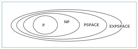
Till now, we have not discussed P and NP classes in this tutorial. These will be discussed later.
Design and Analysis Divide and Conquer
Many algorithms are recursive in nature to solve a given problem recursively dealing with sub-problems.
In divide and conquer approach, a problem is divided into smaller problems, then the smaller problems are solved independently, and finally the solutions of smaller problems are combined into a solution for the large problem.
Generally, divide-and-conquer algorithms have three parts −
-
Divide the problem into a number of sub-problems that are smaller instances of the same problem.
-
Conquer the sub-problems by solving them recursively. If they are small enough, solve the sub-problems as base cases.
-
Combine the solutions to the sub-problems into the solution for the original problem.
Pros and cons of Divide and Conquer Approach
Divide and conquer approach supports parallelism as sub-problems are independent. Hence, an algorithm, which is designed using this technique, can run on the multiprocessor system or in different machines simultaneously.
In this approach, most of the algorithms are designed using recursion, hence memory management is very high. For recursive function stack is used, where function state needs to be stored.
Application of Divide and Conquer Approach
Following are some problems, which are solved using divide and conquer approach.
- Finding the maximum and minimum of a sequence of numbers
- Strassen's matrix multiplication
- Merge sort
- Binary search
Design and Analysis Max-Min Problem
Let us consider a simple problem that can be solved by divide and conquer technique.
Problem Statement
The Max-Min Problem in algorithm analysis is finding the maximum and minimum value in an array.
Solution
To find the maximum and minimum numbers in a given array numbers[] of size n, the following algorithm can be used. First we are representing the naive method and then we will present divide and conquer approach.
Naïve Method
Naïve method is a basic method to solve any problem. In this method, the maximum and minimum number can be found separately. To find the maximum and minimum numbers, the following straightforward algorithm can be used.
Algorithm: Max-Min-Element (numbers[]) max := numbers[1] min := numbers[1] for i = 2 to n do if numbers[i] > max then max := numbers[i] if numbers[i] < min then min := numbers[i] return (max, min)
Analysis
The number of comparison in Naive method is 2n - 2.
The number of comparisons can be reduced using the divide and conquer approach. Following is the technique.
Divide and Conquer Approach
In this approach, the array is divided into two halves. Then using recursive approach maximum and minimum numbers in each halves are found. Later, return the maximum of two maxima of each half and the minimum of two minima of each half.
In this given problem, the number of elements in an array is $y - x + 1$, where y is greater than or equal to x.
$\mathbf{\mathit{Max - Min(x, y)}}$ will return the maximum and minimum values of an array $\mathbf{\mathit{numbers[x...y]}}$.
Algorithm: Max - Min(x, y) if y – x ≤ 1 then return (max(numbers[x], numbers[y]), min((numbers[x], numbers[y])) else (max1, min1):= maxmin(x, ⌊((x + y)/2)⌋) (max2, min2):= maxmin(⌊((x + y)/2) + 1)⌋,y) return (max(max1, max2), min(min1, min2))
Analysis
Let T(n) be the number of comparisons made by $\mathbf{\mathit{Max - Min(x, y)}}$, where the number of elements $n = y - x + 1$.
If T(n) represents the numbers, then the recurrence relation can be represented as
$$T(n) = \begin{cases}T\left(\lfloor\frac{n}{2}\rfloor\right)+T\left(\lceil\frac{n}{2}\rceil\right)+2 & for\: n>2\\1 & for\:n = 2 \\0 & for\:n = 1\end{cases}$$
Let us assume that n is in the form of power of 2. Hence, n = 2k where k is height of the recursion tree.
So,
$$T(n) = 2.T (\frac{n}{2}) + 2 = 2.\left(\begin{array}{c}2.T(\frac{n}{4}) + 2\end{array}\right) + 2 ..... = \frac{3n}{2} - 2$$
Compared to Naïve method, in divide and conquer approach, the number of comparisons is less. However, using the asymptotic notation both of the approaches are represented by O(n).
Design and Analysis Merge Sort
In this chapter, we will discuss merge sort and analyze its complexity.
Problem Statement
The problem of sorting a list of numbers lends itself immediately to a divide-and-conquer strategy: split the list into two halves, recursively sort each half, and then merge the two sorted sub-lists.
Solution
In this algorithm, the numbers are stored in an array numbers[] . Here, p and q represents the start and end index of a sub-array.
Algorithm: Merge-Sort (numbers[], p, r) if p < r then q = ⌊(p + r) / 2⌋ Merge-Sort (numbers[], p, q) Merge-Sort (numbers[], q + 1, r) Merge (numbers[], p, q, r)
Function: Merge (numbers[], p, q, r) n1 = q – p + 1 n2 = r – q declare leftnums[1…n1 + 1] and rightnums[1…n2 + 1] temporary arrays for i = 1 to n1 leftnums[i] = numbers[p + i - 1] for j = 1 to n2 rightnums[j] = numbers[q+ j] leftnums[n1 + 1] = ∞ rightnums[n2 + 1] = ∞ i = 1 j = 1 for k = p to r if leftnums[i] ≤ rightnums[j] numbers[k] = leftnums[i] i = i + 1 else numbers[k] = rightnums[j] j = j + 1
Analysis
Let us consider, the running time of Merge-Sort as T(n) . Hence,
$T(n)=\begin{cases}c & if\:n\leqslant 1\\2\:x\:T(\frac{n}{2})+d\:x\:n & otherwise\end{cases}$ where c and d are constants
Therefore, using this recurrence relation,
$$T(n) = 2^i T(\frac{n}{2^i}) + i.d.n$$
As, $i = log\:n,\: T(n) = 2^{log\:n} T(\frac{n}{2^{log\:n}}) + log\:n.d.n$
$=\:c.n + d.n.log\:n$
Therefore, $T(n) = O(n\:log\:n)$
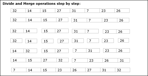
Example
In the following example, we have shown Merge-Sort algorithm step by step. First, every iteration array is divided into two sub-arrays, until the sub-array contains only one element. When these sub-arrays cannot be divided further, then merge operations are performed.
Design and Analysis Binary Search
In this chapter, we will discuss another algorithm based on divide and conquer method.
Problem Statement
Binary search can be performed on a sorted array. In this approach, the index of an element x is determined if the element belongs to the list of elements. If the array is unsorted, linear search is used to determine the position.
Solution
In this algorithm, we want to find whether element x belongs to a set of numbers stored in an array numbers[] . Where l and r represent the left and right index of a sub-array in which searching operation should be performed.
Algorithm: Binary-Search(numbers[], x, l, r) if l = r then return l else m := ⌊(l + r) / 2⌋ if x ≤ numbers[m] then return Binary-Search(numbers[], x, l, m) else return Binary-Search(numbers[], x, m+1, r)
Analysis
Linear search runs in O(n) time. Whereas binary search produces the result in O(log n) time
Let T(n) be the number of comparisons in worst-case in an array of n elements.
Hence,
$$T(n)=\begin{cases}0 & if\:n= 1\\T(\frac{n}{2})+1 & otherwise\end{cases}$$
Using this recurrence relation $T(n) = log\:n$.
Therefore, binary search uses $O(log\:n)$ time.
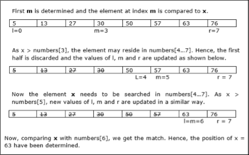
Example
In this example, we are going to search element 63.
Design and Analysis Strassen's Matrix Multiplication
In this chapter, first we will discuss the general method of matrix multiplication and later we will discuss Strassen's matrix multiplication algorithm.
Problem Statement
Let us consider two matrices X and Y . We want to calculate the resultant matrix Z by multiplying X and Y .
Naïve Method
First, we will discuss naïve method and its complexity. Here, we are calculating Z = X × Y . Using Naïve method, two matrices ( X and Y ) can be multiplied if the order of these matrices are p × q and q × r . Following is the algorithm.
Algorithm: Matrix-Multiplication (X, Y, Z) for i = 1 to p do for j = 1 to r do Z[i,j] := 0 for k = 1 to q do Z[i,j] := Z[i,j] + X[i,k] × Y[k,j]
Complexity
Here, we assume that integer operations take O(1) time. There are three for loops in this algorithm and one is nested in other. Hence, the algorithm takes O(n3) time to execute.
Strassen's Matrix Multiplication Algorithm
In this context, using Strassen's Matrix multiplication algorithm, the time consumption can be improved a little bit.
Strassen's Matrix multiplication can be performed only on square matrices where n is a power of 2. Order of both of the matrices are n × n.
Divide X, Y and Z into four (n/2)×(n/2) matrices as represented below −
$Z = \begin{bmatrix}I & J \\K & L \end{bmatrix}$ $X = \begin{bmatrix}A & B \\C & D \end{bmatrix}$ and $Y = \begin{bmatrix}E & F \\G & H \end{bmatrix}$
Using Strassen's Algorithm compute the following −
$$M_{1} \: \colon= (A+C) \times (E+F)$$
$$M_{2} \: \colon= (B+D) \times (G+H)$$
$$M_{3} \: \colon= (A-D) \times (E+H)$$
$$M_{4} \: \colon= A \times (F-H)$$
$$M_{5} \: \colon= (C+D) \times (E)$$
$$M_{6} \: \colon= (A+B) \times (H)$$
$$M_{7} \: \colon= D \times (G-E)$$
Then,
$$I \: \colon= M_{2} + M_{3} - M_{6} - M_{7}$$
$$J \: \colon= M_{4} + M_{6}$$
$$K \: \colon= M_{5} + M_{7}$$
$$L \: \colon= M_{1} - M_{3} - M_{4} - M_{5}$$
Analysis
$T(n)=\begin{cases}c & if\:n= 1\\7\:x\:T(\frac{n}{2})+d\:x\:n^2 & otherwise\end{cases}$ where c and d are constants
Using this recurrence relation, we get $T(n) = O(n^{log7})$
Hence, the complexity of Strassen's matrix multiplication algorithm is $O(n^{log7})$.
Design and Analysis Greedy Method
Among all the algorithmic approaches, the simplest and straightforward approach is the Greedy method. In this approach, the decision is taken on the basis of current available information without worrying about the effect of the current decision in future.
Greedy algorithms build a solution part by part, choosing the next part in such a way, that it gives an immediate benefit. This approach never reconsiders the choices taken previously. This approach is mainly used to solve optimization problems. Greedy method is easy to implement and quite efficient in most of the cases. Hence, we can say that Greedy algorithm is an algorithmic paradigm based on heuristic that follows local optimal choice at each step with the hope of finding global optimal solution.
In many problems, it does not produce an optimal solution though it gives an approximate (near optimal) solution in a reasonable time.
Components of Greedy Algorithm
Greedy algorithms have the following five components −
-
A candidate set − A solution is created from this set.
-
A selection function − Used to choose the best candidate to be added to the solution.
-
A feasibility function − Used to determine whether a candidate can be used to contribute to the solution.
-
An objective function − Used to assign a value to a solution or a partial solution.
-
A solution function − Used to indicate whether a complete solution has been reached.
Areas of Application
Greedy approach is used to solve many problems, such as
-
Finding the shortest path between two vertices using Dijkstra's algorithm.
-
Finding the minimal spanning tree in a graph using Prim's /Kruskal's algorithm, etc.
Where Greedy Approach Fails
In many problems, Greedy algorithm fails to find an optimal solution, moreover it may produce a worst solution. Problems like Travelling Salesman and Knapsack cannot be solved using this approach.
Design and Analysis Fractional Knapsack
The Greedy algorithm could be understood very well with a well-known problem referred to as Knapsack problem. Although the same problem could be solved by employing other algorithmic approaches, Greedy approach solves Fractional Knapsack problem reasonably in a good time. Let us discuss the Knapsack problem in detail.
Knapsack Problem
Given a set of items, each with a weight and a value, determine a subset of items to include in a collection so that the total weight is less than or equal to a given limit and the total value is as large as possible.
The knapsack problem is in combinatorial optimization problem. It appears as a subproblem in many, more complex mathematical models of real-world problems. One general approach to difficult problems is to identify the most restrictive constraint, ignore the others, solve a knapsack problem, and somehow adjust the solution to satisfy the ignored constraints.
Applications
In many cases of resource allocation along with some constraint, the problem can be derived in a similar way of Knapsack problem. Following is a set of example.
- Finding the least wasteful way to cut raw materials
- portfolio optimization
- Cutting stock problems
Problem Scenario
A thief is robbing a store and can carry a maximal weight of W into his knapsack. There are n items available in the store and weight of ith item is wi and its profit is pi . What items should the thief take?
In this context, the items should be selected in such a way that the thief will carry those items for which he will gain maximum profit. Hence, the objective of the thief is to maximize the profit.
Based on the nature of the items, Knapsack problems are categorized as
- Fractional Knapsack
- Knapsack
Fractional Knapsack
In this case, items can be broken into smaller pieces, hence the thief can select fractions of items.
According to the problem statement,
-
There are n items in the store
-
Weight of ith item $w_{i} > 0$
-
Profit for ith item $p_{i} > 0$ and
-
Capacity of the Knapsack is W
In this version of Knapsack problem, items can be broken into smaller pieces. So, the thief may take only a fraction xi of ith item.
$$0 \leqslant x_{i} \leqslant 1$$
The ith item contributes the weight $x_{i}.w_{i}$ to the total weight in the knapsack and profit $x_{i}.p_{i}$ to the total profit.
Hence, the objective of this algorithm is to
$$maximize\:\displaystyle\sum\limits_{n=1}^n (x_{i}.p_{}i)$$
subject to constraint,
$$\displaystyle\sum\limits_{n=1}^n (x_{i}.w_{}i) \leqslant W$$
It is clear that an optimal solution must fill the knapsack exactly, otherwise we could add a fraction of one of the remaining items and increase the overall profit.
Thus, an optimal solution can be obtained by
$$\displaystyle\sum\limits_{n=1}^n (x_{i}.w_{}i) = W$$
In this context, first we need to sort those items according to the value of $\frac{p_{i}}{w_{i}}$, so that $\frac{p_{i}+1}{w_{i}+1}$ ≤ $\frac{p_{i}}{w_{i}}$ . Here, x is an array to store the fraction of items.
Algorithm: Greedy-Fractional-Knapsack (w[1..n], p[1..n], W) for i = 1 to n do x[i] = 0 weight = 0 for i = 1 to n if weight + w[i] ≤ W then x[i] = 1 weight = weight + w[i] else x[i] = (W - weight) / w[i] weight = W break return x
Analysis
If the provided items are already sorted into a decreasing order of $\mathbf{\frac{p_{i}}{w_{i}}}$, then the whileloop takes a time in O(n) ; Therefore, the total time including the sort is in O(n logn) .
Example
Let us consider that the capacity of the knapsack W = 60 and the list of provided items are shown in the following table −
| Item | A | B | C | D |
|---|---|---|---|---|
| Profit | 280 | 100 | 120 | 120 |
| Weight | 40 | 10 | 20 | 24 |
| Ratio $(\frac{p_{i}}{w_{i}})$ | 7 | 10 | 6 | 5 |
As the provided items are not sorted based on $\mathbf{\frac{p_{i}}{w_{i}}}$. After sorting, the items are as shown in the following table.
| Item | B | A | C | D |
|---|---|---|---|---|
| Profit | 100 | 280 | 120 | 120 |
| Weight | 10 | 40 | 20 | 24 |
| Ratio $(\frac{p_{i}}{w_{i}})$ | 10 | 7 | 6 | 5 |
Solution
After sorting all the items according to $\frac{p_{i}}{w_{i}}$. First all of B is chosen as weight of B is less than the capacity of the knapsack. Next, item A is chosen, as the available capacity of the knapsack is greater than the weight of A . Now, C is chosen as the next item. However, the whole item cannot be chosen as the remaining capacity of the knapsack is less than the weight of C .
Hence, fraction of C (i.e. (60 − 50)/20) is chosen.
Now, the capacity of the Knapsack is equal to the selected items. Hence, no more item can be selected.
The total weight of the selected items is 10 + 40 + 20 * (10/20) = 60
And the total profit is 100 + 280 + 120 * (10/20) = 380 + 60 = 440
This is the optimal solution. We cannot gain more profit selecting any different combination of items.
Job Sequencing with Deadline
Problem Statement
In job sequencing problem, the objective is to find a sequence of jobs, which is completed within their deadlines and gives maximum profit.
Solution
Let us consider, a set of n given jobs which are associated with deadlines and profit is earned, if a job is completed by its deadline. These jobs need to be ordered in such a way that there is maximum profit.
It may happen that all of the given jobs may not be completed within their deadlines.
Assume, deadline of ith job Ji is di and the profit received from this job is pi . Hence, the optimal solution of this algorithm is a feasible solution with maximum profit.
Thus, $D(i) > 0$ for $1 \leqslant i \leqslant n$.
Initially, these jobs are ordered according to profit, i.e. $p_{1} \geqslant p_{2} \geqslant p_{3} \geqslant \:... \: \geqslant p_{n}$.
Algorithm: Job-Sequencing-With-Deadline (D, J, n, k) D(0) := J(0) := 0 k := 1 J(1) := 1 // means first job is selected for i = 2 … n do r := k while D(J(r)) > D(i) and D(J(r)) ≠ r do r := r – 1 if D(J(r)) ≤ D(i) and D(i) > r then for l = k … r + 1 by -1 do J(l + 1) := J(l) J(r + 1) := i k := k + 1
Analysis
In this algorithm, we are using two loops, one is within another. Hence, the complexity of this algorithm is $O(n^2)$.
Example
Let us consider a set of given jobs as shown in the following table. We have to find a sequence of jobs, which will be completed within their deadlines and will give maximum profit. Each job is associated with a deadline and profit.
| Job | J1 | J2 | J3 | J4 | J5 |
|---|---|---|---|---|---|
| Deadline | 2 | 1 | 3 | 2 | 1 |
| Profit | 60 | 100 | 20 | 40 | 20 |
Solution
To solve this problem, the given jobs are sorted according to their profit in a descending order. Hence, after sorting, the jobs are ordered as shown in the following table.
| Job | J2 | J1 | J4 | J3 | J5 |
|---|---|---|---|---|---|
| Deadline | 1 | 2 | 2 | 3 | 1 |
| Profit | 100 | 60 | 40 | 20 | 20 |
From this set of jobs, first we select J2 , as it can be completed within its deadline and contributes maximum profit.
-
Next, J1 is selected as it gives more profit compared to J4 .
-
In the next clock, J4 cannot be selected as its deadline is over, hence J3 is selected as it executes within its deadline.
-
The job J5 is discarded as it cannot be executed within its deadline.
Thus, the solution is the sequence of jobs ( J2, J1, J3 ), which are being executed within their deadline and gives maximum profit.
Total profit of this sequence is 100 + 60 + 20 = 180.
Design and Analysis Optimal Merge Pattern
Merge a set of sorted files of different length into a single sorted file. We need to find an optimal solution, where the resultant file will be generated in minimum time.
If the number of sorted files are given, there are many ways to merge them into a single sorted file. This merge can be performed pair wise. Hence, this type of merging is called as 2-way merge patterns.
As, different pairings require different amounts of time, in this strategy we want to determine an optimal way of merging many files together. At each step, two shortest sequences are merged.
To merge a p-record file and a q-record file requires possibly p + q record moves, the obvious choice being, merge the two smallest files together at each step.
Two-way merge patterns can be represented by binary merge trees. Let us consider a set of n sorted files {f1, f2, f3, …, fn}. Initially, each element of this is considered as a single node binary tree. To find this optimal solution, the following algorithm is used.
Algorithm: TREE (n) for i := 1 to n – 1 do declare new node node.leftchild := least (list) node.rightchild := least (list) node.weight) := ((node.leftchild).weight) + ((node.rightchild).weight) insert (list, node); return least (list);
At the end of this algorithm, the weight of the root node represents the optimal cost.
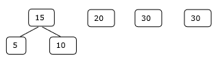
Example
Let us consider the given files, f1, f2, f3, f4 and f5 with 20, 30, 10, 5 and 30 number of elements respectively.
If merge operations are performed according to the provided sequence, then
M1 = merge f1 and f2 => 20 + 30 = 50
M2 = merge M1 and f3 => 50 + 10 = 60
M3 = merge M2 and f4 => 60 + 5 = 65
M4 = merge M3 and f5 => 65 + 30 = 95
Hence, the total number of operations is
50 + 60 + 65 + 95 = 270
Now, the question arises is there any better solution?
Sorting the numbers according to their size in an ascending order, we get the following sequence −
f4, f3, f1, f2, f5
Hence, merge operations can be performed on this sequence
M1 = merge f4 and f3 => 5 + 10 = 15
M2 = merge M1 and f1 => 15 + 20 = 35
M3 = merge M2 and f2 => 35 + 30 = 65
M4 = merge M3 and f5 => 65 + 30 = 95
Therefore, the total number of operations is
15 + 35 + 65 + 95 = 210
Obviously, this is better than the previous one.
In this context, we are now going to solve the problem using this algorithm.
Initial Set
Step-1
Step-2
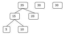
Step-3
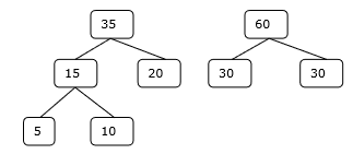
Step-4
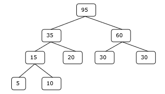
Hence, the solution takes 15 + 35 + 60 + 95 = 205 number of comparisons.
Design and Analysis Dynamic Programming
Dynamic Programming is also used in optimization problems. Like divide-and-conquer method, Dynamic Programming solves problems by combining the solutions of subproblems. Moreover, Dynamic Programming algorithm solves each sub-problem just once and then saves its answer in a table, thereby avoiding the work of re-computing the answer every time.
Two main properties of a problem suggest that the given problem can be solved using Dynamic Programming. These properties are overlapping sub-problems and optimal substructure.
Overlapping Sub-Problems
Similar to Divide-and-Conquer approach, Dynamic Programming also combines solutions to sub-problems. It is mainly used where the solution of one sub-problem is needed repeatedly. The computed solutions are stored in a table, so that these don't have to be re-computed. Hence, this technique is needed where overlapping sub-problem exists.
For example, Binary Search does not have overlapping sub-problem. Whereas recursive program of Fibonacci numbers have many overlapping sub-problems.
Optimal Sub-Structure
A given problem has Optimal Substructure Property, if the optimal solution of the given problem can be obtained using optimal solutions of its sub-problems.
For example, the Shortest Path problem has the following optimal substructure property −
If a node x lies in the shortest path from a source node u to destination node v, then the shortest path from u to v is the combination of the shortest path from u to x, and the shortest path from x to v.
The standard All Pair Shortest Path algorithms like Floyd-Warshall and Bellman-Ford are typical examples of Dynamic Programming.
Steps of Dynamic Programming Approach
Dynamic Programming algorithm is designed using the following four steps −
- Characterize the structure of an optimal solution.
- Recursively define the value of an optimal solution.
- Compute the value of an optimal solution, typically in a bottom-up fashion.
- Construct an optimal solution from the computed information.
Applications of Dynamic Programming Approach
- Matrix Chain Multiplication
- Longest Common Subsequence
- Travelling Salesman Problem
Design and Analysis 0-1 Knapsack
In this tutorial, earlier we have discussed Fractional Knapsack problem using Greedy approach. We have shown that Greedy approach gives an optimal solution for Fractional Knapsack. However, this chapter will cover 0-1 Knapsack problem and its analysis.
In 0-1 Knapsack, items cannot be broken which means the thief should take the item as a whole or should leave it. This is reason behind calling it as 0-1 Knapsack.
Hence, in case of 0-1 Knapsack, the value of xi can be either 0 or 1 , where other constraints remain the same.
0-1 Knapsack cannot be solved by Greedy approach. Greedy approach does not ensure an optimal solution. In many instances, Greedy approach may give an optimal solution.
The following examples will establish our statement.
Example-1
Let us consider that the capacity of the knapsack is W = 25 and the items are as shown in the following table.
| Item | A | B | C | D |
|---|---|---|---|---|
| Profit | 24 | 18 | 18 | 10 |
| Weight | 24 | 10 | 10 | 7 |
Without considering the profit per unit weight ( pi/wi ), if we apply Greedy approach to solve this problem, first item A will be selected as it will contribute maximum profit among all the elements.
After selecting item A , no more item will be selected. Hence, for this given set of items total profit is 24 . Whereas, the optimal solution can be achieved by selecting items, B and C, where the total profit is 18 + 18 = 36.
Example-2
Instead of selecting the items based on the overall benefit, in this example the items are selected based on ratio pi/wi . Let us consider that the capacity of the knapsack is W = 60 and the items are as shown in the following table.
| Item | A | B | C |
|---|---|---|---|
| Price | 100 | 280 | 120 |
| Weight | 10 | 40 | 20 |
| Ratio | 10 | 7 | 6 |
Using the Greedy approach, first item A is selected. Then, the next item B is chosen. Hence, the total profit is 100 + 280 = 380. However, the optimal solution of this instance can be achieved by selecting items, B and C , where the total profit is 280 + 120 = 400.
Hence, it can be concluded that Greedy approach may not give an optimal solution.
To solve 0-1 Knapsack, Dynamic Programming approach is required.
Problem Statement
A thief is robbing a store and can carry a maximal weight of W into his knapsack. There are n items and weight of ith item is wi and the profit of selecting this item is pi . What items should the thief take?
Dynamic-Programming Approach
Let i be the highest-numbered item in an optimal solution S for W dollars. Then S' = S - {i} is an optimal solution for W - wi dollars and the value to the solution S is Vi plus the value of the sub-problem.
We can express this fact in the following formula: define c[i, w] to be the solution for items 1,2, … , i and the maximum weight w.
The algorithm takes the following inputs
-
The maximum weight W
-
The number of items n
-
The two sequences v = <v1, v2, …, vn> and w = <w1, w2, …, wn>
Dynamic-0-1-knapsack (v, w, n, W) for w = 0 to W do c[0, w] = 0 for i = 1 to n do c[i, 0] = 0 for w = 1 to W do if wi ≤ w then if vi + c[i-1, w-wi] then c[i, w] = vi + c[i-1, w-wi] else c[i, w] = c[i-1, w] else c[i, w] = c[i-1, w]
The set of items to take can be deduced from the table, starting at c[n, w] and tracing backwards where the optimal values came from.
If c[i, w] = c[i-1, w], then item i is not part of the solution, and we continue tracing with c[i-1, w]. Otherwise, item i is part of the solution, and we continue tracing with c[i-1, w-W].
Analysis
This algorithm takes θ(n, w) times as table c has (n + 1).(w + 1) entries, where each entry requires θ(1) time to compute.
Longest Common Subsequence
The longest common subsequence problem is finding the longest sequence which exists in both the given strings.
Subsequence
Let us consider a sequence S = <s1, s2, s3, s4, …,sn>.
A sequence Z = <z1, z2, z3, z4, …,zm> over S is called a subsequence of S, if and only if it can be derived from S deletion of some elements.
Common Subsequence
Suppose, X and Y are two sequences over a finite set of elements. We can say that Z is a common subsequence of X and Y , if Z is a subsequence of both X and Y .
Longest Common Subsequence
If a set of sequences are given, the longest common subsequence problem is to find a common subsequence of all the sequences that is of maximal length.
The longest common subsequence problem is a classic computer science problem, the basis of data comparison programs such as the diff-utility, and has applications in bioinformatics. It is also widely used by revision control systems, such as SVN and Git, for reconciling multiple changes made to a revision-controlled collection of files.
Naïve Method
Let X be a sequence of length m and Y a sequence of length n . Check for every subsequence of X whether it is a subsequence of Y , and return the longest common subsequence found.
There are 2m subsequences of X . Testing sequences whether or not it is a subsequence of Y takes O(n) time. Thus, the naïve algorithm would take O(n2m) time.
Dynamic Programming
Let X = < x1, x2, x3,…, xm > and Y = < y1, y2, y3,…, yn > be the sequences. To compute the length of an element the following algorithm is used.
In this procedure, table C[m, n] is computed in row major order and another table B[m,n] is computed to construct optimal solution.
Algorithm: LCS-Length-Table-Formulation (X, Y) m := length(X) n := length(Y) for i = 1 to m do C[i, 0] := 0 for j = 1 to n do C[0, j] := 0 for i = 1 to m do for j = 1 to n do if xi = yj C[i, j] := C[i - 1, j - 1] + 1 B[i, j] := 'D' else if C[i -1, j] ≥ C[i, j -1] C[i, j] := C[i - 1, j] + 1 B[i, j] := 'U' else C[i, j] := C[i, j - 1] B[i, j] := 'L' return C and B
Algorithm: Print-LCS (B, X, i, j) if i = 0 and j = 0 return if B[i, j] = 'D' Print-LCS(B, X, i-1, j-1) Print(xi) else if B[i, j] = 'U' Print-LCS(B, X, i-1, j) else Print-LCS(B, X, i, j-1)
This algorithm will print the longest common subsequence of X and Y.
Analysis
To populate the table, the outer for loop iterates m times and the inner for loop iterates n times. Hence, the complexity of the algorithm is O(m, n), where m and n are the length of two strings.
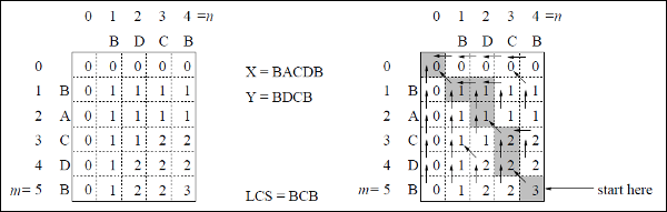
Example
In this example, we have two strings X = BACDB and Y = BDCB to find the longest common subsequence.
Following the algorithm LCS-Length-Table-Formulation (as stated above), we have calculated table C (shown on the left hand side) and table B (shown on the right hand side).
In table B, instead of 'D', 'L' and 'U', we are using the diagonal arrow, left arrow and up arrow, respectively. After generating table B, the LCS is determined by function LCS-Print. The result is BCB.
Design and Analysis Spanning Tree
A spanning tree is a subset of an undirected Graph that has all the vertices connected by minimum number of edges.
If all the vertices are connected in a graph, then there exists at least one spanning tree. In a graph, there may exist more than one spanning tree.
Properties
- A spanning tree does not have any cycle.
- Any vertex can be reached from any other vertex.
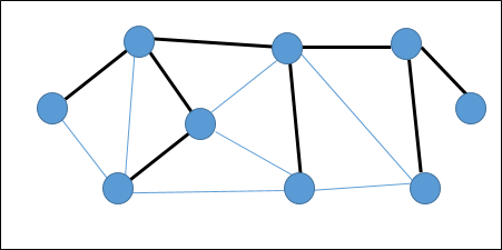
Example
In the following graph, the highlighted edges form a spanning tree.
Minimum Spanning Tree
A Minimum Spanning Tree (MST) is a subset of edges of a connected weighted undirected graph that connects all the vertices together with the minimum possible total edge weight. To derive an MST, Prim's algorithm or Kruskal's algorithm can be used. Hence, we will discuss Prim's algorithm in this chapter.
As we have discussed, one graph may have more than one spanning tree. If there are n number of vertices, the spanning tree should have n - 1 number of edges. In this context, if each edge of the graph is associated with a weight and there exists more than one spanning tree, we need to find the minimum spanning tree of the graph.
Moreover, if there exist any duplicate weighted edges, the graph may have multiple minimum spanning tree.
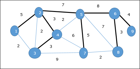
In the above graph, we have shown a spanning tree though it's not the minimum spanning tree. The cost of this spanning tree is (5 + 7 + 3 + 3 + 5 + 8 + 3 + 4) = 38.
We will use Prim's algorithm to find the minimum spanning tree.
Prim's Algorithm
Prim's algorithm is a greedy approach to find the minimum spanning tree. In this algorithm, to form a MST we can start from an arbitrary vertex.
Algorithm: MST-Prim's (G, w, r) for each u є G.V u.key = ∞ u.∏ = NIL r.key = 0 Q = G.V while Q ≠ Ф u = Extract-Min (Q) for each v є G.adj[u] if each v є Q and w(u, v) < v.key v.∏ = u v.key = w(u, v)
The function Extract-Min returns the vertex with minimum edge cost. This function works on min-heap.
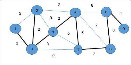
Example
Using Prim's algorithm, we can start from any vertex, let us start from vertex 1.
Vertex 3 is connected to vertex 1 with minimum edge cost, hence edge (1, 2) is added to the spanning tree.
Next, edge (2, 3) is considered as this is the minimum among edges {(1, 2), (2, 3), (3, 4), (3, 7)}.
In the next step, we get edge (3, 4) and (2, 4) with minimum cost. Edge (3, 4) is selected at random.
In a similar way, edges (4, 5), (5, 7), (7, 8), (6, 8) and (6, 9) are selected. As all the vertices are visited, now the algorithm stops.
The cost of the spanning tree is (2 + 2 + 3 + 2 + 5 + 2 + 3 + 4) = 23. There is no more spanning tree in this graph with cost less than 23.
Design and Analysis Shortest Paths
Dijkstra's Algorithm
Dijkstra's algorithm solves the single-source shortest-paths problem on a directed weighted graph G = (V, E), where all the edges are non-negative (i.e., w(u, v) ≥ 0 for each edge (u, v) Є E).
In the following algorithm, we will use one function Extract-Min() , which extracts the node with the smallest key.
Algorithm: Dijkstra's-Algorithm (G, w, s) for each vertex v Є G.V v.d := ∞ v.∏ := NIL s.d := 0 S := Ф Q := G.V while Q ≠ Ф u := Extract-Min (Q) S := S U {u} for each vertex v Є G.adj[u] if v.d > u.d + w(u, v) v.d := u.d + w(u, v) v.∏ := u Analysis
The complexity of this algorithm is fully dependent on the implementation of Extract-Min function. If extract min function is implemented using linear search, the complexity of this algorithm is O(V2 + E) .
In this algorithm, if we use min-heap on which Extract-Min() function works to return the node from Q with the smallest key, the complexity of this algorithm can be reduced further.
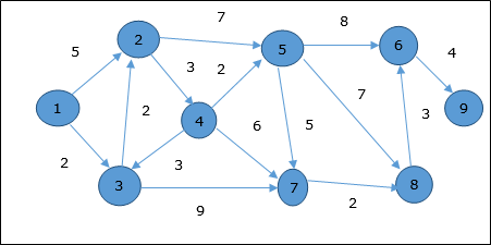
Example
Let us consider vertex 1 and 9 as the start and destination vertex respectively. Initially, all the vertices except the start vertex are marked by ∞ and the start vertex is marked by 0 .
| Vertex | Initial | Step1 V1 | Step2 V3 | Step3 V2 | Step4 V4 | Step5 V5 | Step6 V7 | Step7 V8 | Step8 V6 |
|---|---|---|---|---|---|---|---|---|---|
| 1 | 0 | 0 | 0 | 0 | 0 | 0 | 0 | 0 | 0 |
| 2 | ∞ | 5 | 4 | 4 | 4 | 4 | 4 | 4 | 4 |
| 3 | ∞ | 2 | 2 | 2 | 2 | 2 | 2 | 2 | 2 |
| 4 | ∞ | ∞ | ∞ | 7 | 7 | 7 | 7 | 7 | 7 |
| 5 | ∞ | ∞ | ∞ | 11 | 9 | 9 | 9 | 9 | 9 |
| 6 | ∞ | ∞ | ∞ | ∞ | ∞ | 17 | 17 | 16 | 16 |
| 7 | ∞ | ∞ | 11 | 11 | 11 | 11 | 11 | 11 | 11 |
| 8 | ∞ | ∞ | ∞ | ∞ | ∞ | 16 | 13 | 13 | 13 |
| 9 | ∞ | ∞ | ∞ | ∞ | ∞ | ∞ | ∞ | ∞ | 20 |
Hence, the minimum distance of vertex 9 from vertex 1 is 20 . And the path is
1→ 3→ 7→ 8→ 6→ 9
This path is determined based on predecessor information.
Bellman Ford Algorithm
This algorithm solves the single source shortest path problem of a directed graph G = (V, E) in which the edge weights may be negative. Moreover, this algorithm can be applied to find the shortest path, if there does not exist any negative weighted cycle.
Algorithm: Bellman-Ford-Algorithm (G, w, s) for each vertex v Є G.V v.d := ∞ v.∏ := NIL s.d := 0 for i = 1 to |G.V| - 1 for each edge (u, v) Є G.E if v.d > u.d + w(u, v) v.d := u.d +w(u, v) v.∏ := u for each edge (u, v) Є G.E if v.d > u.d + w(u, v) return FALSE return TRUE
Analysis
The first for loop is used for initialization, which runs in O(V) times. The next for loop runs | V - 1 | passes over the edges, which takes O(E) times.
Hence, Bellman-Ford algorithm runs in O(V, E) time.
Example
The following example shows how Bellman-Ford algorithm works step by step. This graph has a negative edge but does not have any negative cycle, hence the problem can be solved using this technique.
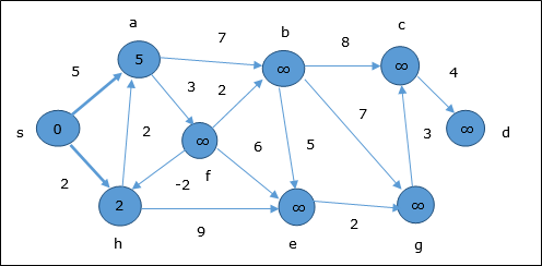
At the time of initialization, all the vertices except the source are marked by ∞ and the source is marked by 0.
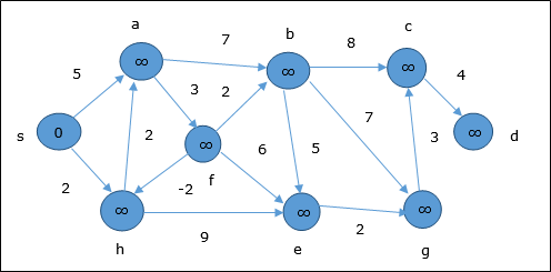
In the first step, all the vertices which are reachable from the source are updated by minimum cost. Hence, vertices a and h are updated.
In the next step, vertices a, b, f and e are updated.
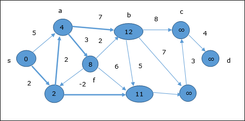
Following the same logic, in this step vertices b, f, c and g are updated.
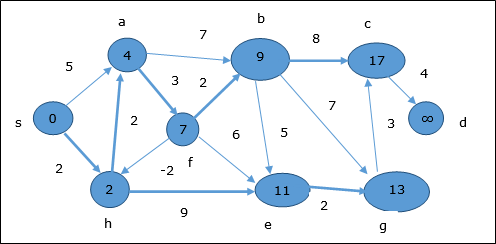
Here, vertices c and d are updated.
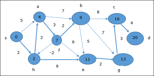
Hence, the minimum distance between vertex s and vertex d is 20.
Based on the predecessor information, the path is s→ h→ e→ g→ c→ d
Design and Analysis Multistage Graph
A multistage graph G = (V, E) is a directed graph where vertices are partitioned into k (where k > 1) number of disjoint subsets S = {s1,s2,…,sk} such that edge (u, v) is in E, then u Є si and v Є s1 + 1 for some subsets in the partition and | s1 | = | sk | = 1.
The vertex s Є s1 is called the source and the vertex t Є sk is called sink.
G is usually assumed to be a weighted graph. In this graph, cost of an edge (i, j) is represented by c(i, j). Hence, the cost of path from source s to sink t is the sum of costs of each edges in this path.
The multistage graph problem is finding the path with minimum cost from source s to sink t .
Example
Consider the following example to understand the concept of multistage graph.
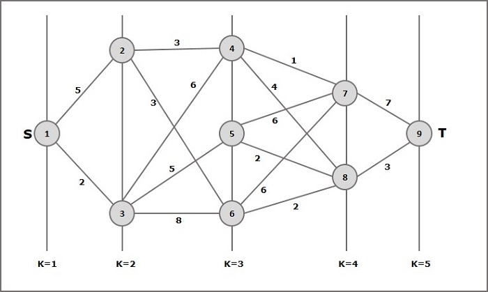
According to the formula, we have to calculate the cost (i, j) using the following steps
Step-1: Cost (K-2, j)
In this step, three nodes (node 4, 5. 6) are selected as j. Hence, we have three options to choose the minimum cost at this step.
Cost(3, 4) = min {c(4, 7) + Cost(7, 9),c(4, 8) + Cost(8, 9)} = 7
Cost(3, 5) = min {c(5, 7) + Cost(7, 9),c(5, 8) + Cost(8, 9)} = 5
Cost(3, 6) = min {c(6, 7) + Cost(7, 9),c(6, 8) + Cost(8, 9)} = 5
Step-2: Cost (K-3, j)
Two nodes are selected as j because at stage k - 3 = 2 there are two nodes, 2 and 3. So, the value i = 2 and j = 2 and 3.
Cost(2, 2) = min {c(2, 4) + Cost(4, 8) + Cost(8, 9),c(2, 6) +
Cost(6, 8) + Cost(8, 9)} = 8
Cost(2, 3) = {c(3, 4) + Cost(4, 8) + Cost(8, 9), c(3, 5) + Cost(5, 8)+ Cost(8, 9), c(3, 6) + Cost(6, 8) + Cost(8, 9)} = 10
Step-3: Cost (K-4, j)
Cost (1, 1) = {c(1, 2) + Cost(2, 6) + Cost(6, 8) + Cost(8, 9), c(1, 3) + Cost(3, 5) + Cost(5, 8) + Cost(8, 9))} = 12
c(1, 3) + Cost(3, 6) + Cost(6, 8 + Cost(8, 9))} = 13
Hence, the path having the minimum cost is 1→ 3→ 5→ 8→ 9.
Travelling Salesman Problem
Problem Statement
A traveler needs to visit all the cities from a list, where distances between all the cities are known and each city should be visited just once. What is the shortest possible route that he visits each city exactly once and returns to the origin city?
Solution
Travelling salesman problem is the most notorious computational problem. We can use brute-force approach to evaluate every possible tour and select the best one. For n number of vertices in a graph, there are (n - 1)! number of possibilities.
Instead of brute-force using dynamic programming approach, the solution can be obtained in lesser time, though there is no polynomial time algorithm.
Let us consider a graph G = (V, E) , where V is a set of cities and E is a set of weighted edges. An edge e(u, v) represents that vertices u and v are connected. Distance between vertex u and v is d(u, v) , which should be non-negative.
Suppose we have started at city 1 and after visiting some cities now we are in city j . Hence, this is a partial tour. We certainly need to know j , since this will determine which cities are most convenient to visit next. We also need to know all the cities visited so far, so that we don't repeat any of them. Hence, this is an appropriate sub-problem.
For a subset of cities S Є {1, 2, 3, ... , n} that includes 1 , and j Є S , let C(S, j) be the length of the shortest path visiting each node in S exactly once, starting at 1 and ending at j .
When | S | > 1, we define C(S, 1) = ∝ since the path cannot start and end at 1.
Now, let express C(S, j) in terms of smaller sub-problems. We need to start at 1 and end at j. We should select the next city in such a way that
$$C(S, j) = min \:C(S - \lbrace j \rbrace, i) + d(i, j)\:where\: i\in S \: and\: i \neq jc(S, j) = minC(s- \lbrace j \rbrace, i)+ d(i,j) \:where\: i\in S \: and\: i \neq j $$
Algorithm: Traveling-Salesman-Problem C ({1}, 1) = 0 for s = 2 to n do for all subsets S Є {1, 2, 3, … , n} of size s and containing 1 C (S, 1) = ∞ for all j Є S and j ≠ 1 C (S, j) = min {C (S – {j}, i) + d(i, j) for i Є S and i ≠ j} Return minj C ({1, 2, 3, …, n}, j) + d(j, i) Analysis
There are at the most $2^n.n$ sub-problems and each one takes linear time to solve. Therefore, the total running time is $O(2^n.n^2)$.
Example
In the following example, we will illustrate the steps to solve the travelling salesman problem.
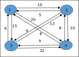
From the above graph, the following table is prepared.
| 1 | 2 | 3 | 4 | |
| 1 | 0 | 10 | 15 | 20 |
| 2 | 5 | 0 | 9 | 10 |
| 3 | 6 | 13 | 0 | 12 |
| 4 | 8 | 8 | 9 | 0 |
S = Φ
$$\small Cost (2,\Phi,1) = d (2,1) = 5\small Cost(2,\Phi,1)=d(2,1)=5$$
$$\small Cost (3,\Phi,1) = d (3,1) = 6\small Cost(3,\Phi,1)=d(3,1)=6$$
$$\small Cost (4,\Phi,1) = d (4,1) = 8\small Cost(4,\Phi,1)=d(4,1)=8$$
S = 1
$$\small Cost (i,s) = min \lbrace Cost (j,s – (j)) + d [i,j]\rbrace\small Cost (i,s)=min \lbrace Cost (j,s)-(j))+ d [i,j]\rbrace$$
$$\small Cost (2,\lbrace 3 \rbrace,1) = d [2,3] + Cost (3,\Phi,1) = 9 + 6 = 15cost(2,\lbrace3 \rbrace,1)=d[2,3]+cost(3,\Phi ,1)=9+6=15$$
$$\small Cost (2,\lbrace 4 \rbrace,1) = d [2,4] + Cost (4,\Phi,1) = 10 + 8 = 18cost(2,\lbrace4 \rbrace,1)=d[2,4]+cost(4,\Phi,1)=10+8=18$$
$$\small Cost (3,\lbrace 2 \rbrace,1) = d [3,2] + Cost (2,\Phi,1) = 13 + 5 = 18cost(3,\lbrace2 \rbrace,1)=d[3,2]+cost(2,\Phi,1)=13+5=18$$
$$\small Cost (3,\lbrace 4 \rbrace,1) = d [3,4] + Cost (4,\Phi,1) = 12 + 8 = 20cost(3,\lbrace4 \rbrace,1)=d[3,4]+cost(4,\Phi,1)=12+8=20$$
$$\small Cost (4,\lbrace 3 \rbrace,1) = d [4,3] + Cost (3,\Phi,1) = 9 + 6 = 15cost(4,\lbrace3 \rbrace,1)=d[4,3]+cost(3,\Phi,1)=9+6=15$$
$$\small Cost (4,\lbrace 2 \rbrace,1) = d [4,2] + Cost (2,\Phi,1) = 8 + 5 = 13cost(4,\lbrace2 \rbrace,1)=d[4,2]+cost(2,\Phi,1)=8+5=13$$
S = 2
$$\small Cost(2, \lbrace 3, 4 \rbrace, 1)=\begin{cases}d[2, 3] + Cost(3, \lbrace 4 \rbrace, 1) = 9 + 20 = 29\\d[2, 4] + Cost(4, \lbrace 3 \rbrace, 1) = 10 + 15 = 25=25\small Cost (2,\lbrace 3,4 \rbrace,1)\\\lbrace d[2,3]+ \small cost(3,\lbrace4\rbrace,1)=9+20=29d[2,4]+ \small Cost (4,\lbrace 3 \rbrace ,1)=10+15=25\end{cases}= 25$$
$$\small Cost(3, \lbrace 2, 4 \rbrace, 1)=\begin{cases}d[3, 2] + Cost(2, \lbrace 4 \rbrace, 1) = 13 + 18 = 31\\d[3, 4] + Cost(4, \lbrace 2 \rbrace, 1) = 12 + 13 = 25=25\small Cost (3,\lbrace 2,4 \rbrace,1)\\\lbrace d[3,2]+ \small cost(2,\lbrace4\rbrace,1)=13+18=31d[3,4]+ \small Cost (4,\lbrace 2 \rbrace ,1)=12+13=25\end{cases}= 25$$
$$\small Cost(4, \lbrace 2, 3 \rbrace, 1)=\begin{cases}d[4, 2] + Cost(2, \lbrace 3 \rbrace, 1) = 8 + 15 = 23\\d[4, 3] + Cost(3, \lbrace 2 \rbrace, 1) = 9 + 18 = 27=23\small Cost (4,\lbrace 2,3 \rbrace,1)\\\lbrace d[4,2]+ \small cost(2,\lbrace3\rbrace,1)=8+15=23d[4,3]+ \small Cost (3,\lbrace 2 \rbrace ,1)=9+18=27\end{cases}= 23$$
S = 3
$$\small Cost(1, \lbrace 2, 3, 4 \rbrace, 1)=\begin{cases}d[1, 2] + Cost(2, \lbrace 3, 4 \rbrace, 1) = 10 + 25 = 35\\d[1, 3] + Cost(3, \lbrace 2, 4 \rbrace, 1) = 15 + 25 = 40\\d[1, 4] + Cost(4, \lbrace 2, 3 \rbrace, 1) = 20 + 23 = 43=35 cost(1,\lbrace 2,3,4 \rbrace),1)\\d[1,2]+cost(2,\lbrace 3,4 \rbrace,1)=10+25=35\\d[1,3]+cost(3,\lbrace 2,4 \rbrace,1)=15+25=40\\d[1,4]+cost(4,\lbrace 2,3 \rbrace ,1)=20+23=43=35\end{cases}$$
The minimum cost path is 35.
Start from cost {1, {2, 3, 4}, 1}, we get the minimum value for d [1, 2]. When s = 3, select the path from 1 to 2 (cost is 10) then go backwards. When s = 2, we get the minimum value for d [4, 2]. Select the path from 2 to 4 (cost is 10) then go backwards.
When s = 1, we get the minimum value for d [4, 3]. Selecting path 4 to 3 (cost is 9), then we shall go to then go to s = Φ step. We get the minimum value for d [3, 1] (cost is 6).

Optimal Cost Binary Search Trees
A Binary Search Tree (BST) is a tree where the key values are stored in the internal nodes. The external nodes are null nodes. The keys are ordered lexicographically, i.e. for each internal node all the keys in the left sub-tree are less than the keys in the node, and all the keys in the right sub-tree are greater.
When we know the frequency of searching each one of the keys, it is quite easy to compute the expected cost of accessing each node in the tree. An optimal binary search tree is a BST, which has minimal expected cost of locating each node
Search time of an element in a BST is O(n) , whereas in a Balanced-BST search time is O(log n) . Again the search time can be improved in Optimal Cost Binary Search Tree, placing the most frequently used data in the root and closer to the root element, while placing the least frequently used data near leaves and in leaves.
Here, the Optimal Binary Search Tree Algorithm is presented. First, we build a BST from a set of provided n number of distinct keys < k1, k2, k3, ... kn > . Here we assume, the probability of accessing a key Ki is pi . Some dummy keys ( d0, d1, d2, ... dn ) are added as some searches may be performed for the values which are not present in the Key set K . We assume, for each dummy key di probability of access is qi .
Optimal-Binary-Search-Tree(p, q, n) e[1…n + 1, 0…n], w[1…n + 1, 0…n], root[1…n + 1, 0…n] for i = 1 to n + 1 do e[i, i - 1] := qi - 1 w[i, i - 1] := qi - 1 for l = 1 to n do for i = 1 to n – l + 1 do j = i + l – 1 e[i, j] := ∞ w[i, i] := w[i, i -1] + pj + qj for r = i to j do t := e[i, r - 1] + e[r + 1, j] + w[i, j] if t < e[i, j] e[i, j] := t root[i, j] := r return e and root
Analysis
The algorithm requires O (n3) time, since three nested for loops are used. Each of these loops takes on at most n values.
Example
Considering the following tree, the cost is 2.80, though this is not an optimal result.
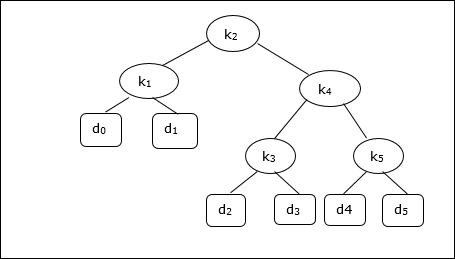
| Node | Depth | Probability | Contribution |
|---|---|---|---|
| k1 | 1 | 0.15 | 0.30 |
| k2 | 0 | 0.10 | 0.10 |
| k3 | 2 | 0.05 | 0.15 |
| k4 | 1 | 0.10 | 0.20 |
| k5 | 2 | 0.20 | 0.60 |
| d0 | 2 | 0.05 | 0.15 |
| d1 | 2 | 0.10 | 0.30 |
| d2 | 3 | 0.05 | 0.20 |
| d3 | 3 | 0.05 | 0.20 |
| d4 | 3 | 0.05 | 0.20 |
| d5 | 3 | 0.10 | 0.40 |
| Total | 2.80 |
To get an optimal solution, using the algorithm discussed in this chapter, the following tables are generated.
In the following tables, column index is i and row index is j.
| e | 1 | 2 | 3 | 4 | 5 | 6 |
|---|---|---|---|---|---|---|
| 5 | 2.75 | 2.00 | 1.30 | 0.90 | 0.50 | 0.10 |
| 4 | 1.75 | 1.20 | 0.60 | 0.30 | 0.05 | |
| 3 | 1.25 | 0.70 | 0.25 | 0.05 | ||
| 2 | 0.90 | 0.40 | 0.05 | |||
| 1 | 0.45 | 0.10 | ||||
| 0 | 0.05 |
| w | 1 | 2 | 3 | 4 | 5 | 6 |
|---|---|---|---|---|---|---|
| 5 | 1.00 | 0.80 | 0.60 | 0.50 | 0.35 | 0.10 |
| 4 | 0.70 | 0.50 | 0.30 | 0.20 | 0.05 | |
| 3 | 0.55 | 0.35 | 0.15 | 0.05 | ||
| 2 | 0.45 | 0.25 | 0.05 | |||
| 1 | 0.30 | 0.10 | ||||
| 0 | 0.05 |
| root | 1 | 2 | 3 | 4 | 5 |
|---|---|---|---|---|---|
| 5 | 2 | 4 | 5 | 5 | 5 |
| 4 | 2 | 2 | 4 | 4 | |
| 3 | 2 | 2 | 3 | ||
| 2 | 1 | 2 | |||
| 1 | 1 |
From these tables, the optimal tree can be formed.
Design and Analysis Binary Heap
There are several types of heaps, however in this chapter, we are going to discuss binary heap. A binary heap is a data structure, which looks similar to a complete binary tree. Heap data structure obeys ordering properties discussed below. Generally, a Heap is represented by an array. In this chapter, we are representing a heap by H .
As the elements of a heap is stored in an array, considering the starting index as 1 , the position of the parent node of ith element can be found at ⌊ i/2 ⌋ . Left child and right child of ith node is at position 2i and 2i + 1 .
A binary heap can be classified further as either a max-heap or a min-heap based on the ordering property.
Max-Heap
In this heap, the key value of a node is greater than or equal to the key value of the highest child.
Hence, H[Parent(i)] ≥ H[i]
Min-Heap
In mean-heap, the key value of a node is lesser than or equal to the key value of the lowest child.
Hence, H[Parent(i)] ≤ H[i]
In this context, basic operations are shown below with respect to Max-Heap. Insertion and deletion of elements in and from heaps need rearrangement of elements. Hence, Heapify function needs to be called.
Array Representation
A complete binary tree can be represented by an array, storing its elements using level order traversal.
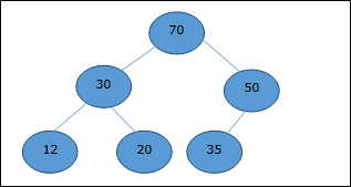
Let us consider a heap (as shown below) which will be represented by an array H.
Considering the starting index as 0, using level order traversal, the elements are being kept in an array as follows.
| Index | 0 | 1 | 2 | 3 | 4 | 5 | 6 | 7 | 8 | ... |
| elements | 70 | 30 | 50 | 12 | 20 | 35 | 25 | 4 | 8 | ... |
In this context, operations on heap are being represented with respect to Max-Heap.
To find the index of the parent of an element at index i, the following algorithm Parent (numbers[], i) is used.
Algorithm: Parent (numbers[], i) if i == 1 return NULL else [i / 2]
The index of the left child of an element at index i can be found using the following algorithm, Left-Child (numbers[], i) .
Algorithm: Left-Child (numbers[], i) If 2 * i ≤ heapsize return [2 * i] else return NULL
The index of the right child of an element at index i can be found using the following algorithm, Right-Child(numbers[], i) .
Algorithm: Right-Child (numbers[], i) if 2 * i < heapsize return [2 * i + 1] else return NULL
Design and Analysis Insert Method
To insert an element in a heap, the new element is initially appended to the end of the heap as the last element of the array.
After inserting this element, heap property may be violated, hence the heap property is repaired by comparing the added element with its parent and moving the added element up a level, swapping positions with the parent. This process is called percolation up .
The comparison is repeated until the parent is larger than or equal to the percolating element.
Algorithm: Max-Heap-Insert (numbers[], key) heapsize = heapsize + 1 numbers[heapsize] = -∞ i = heapsize numbers[i] = key while i > 1 and numbers[Parent(numbers[], i)] < numbers[i] exchange(numbers[i], numbers[Parent(numbers[], i)]) i = Parent (numbers[], i)
Analysis
Initially, an element is being added at the end of the array. If it violates the heap property, the element is exchanged with its parent. The height of the tree is log n . Maximum log n number of operations needs to be performed.
Hence, the complexity of this function is O(log n) .
Example
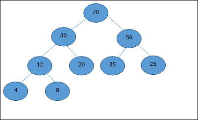
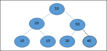
Let us consider a max-heap, as shown below, where a new element 5 needs to be added.
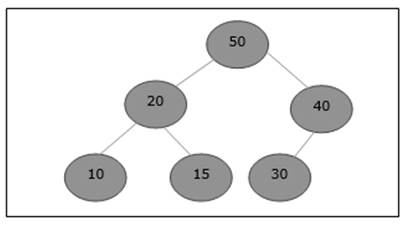
Initially, 55 will be added at the end of this array.
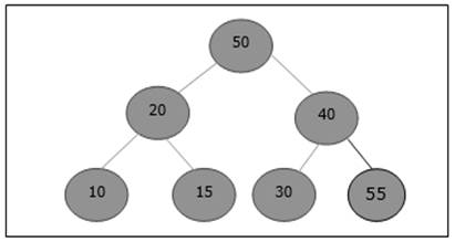
After insertion, it violates the heap property. Hence, the element needs to swap with its parent. After swap, the heap looks like the following.
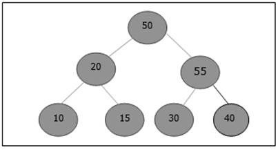
Again, the element violates the property of heap. Hence, it is swapped with its parent.
Now, we have to stop.
Design and Analysis Heapify Method
Heapify method rearranges the elements of an array where the left and right sub-tree of ith element obeys the heap property.
Algorithm: Max-Heapify(numbers[], i) leftchild := numbers[2i] rightchild := numbers [2i + 1] if leftchild ≤ numbers[].size and numbers[leftchild] > numbers[i] largest := leftchild else largest := i if rightchild ≤ numbers[].size and numbers[rightchild] > numbers[largest] largest := rightchild if largest ≠ i swap numbers[i] with numbers[largest] Max-Heapify(numbers, largest)
When the provided array does not obey the heap property, Heap is built based on the following algorithm Build-Max-Heap (numbers[]) .
Algorithm: Build-Max-Heap(numbers[]) numbers[].size := numbers[].length fori = ⌊ numbers[].length/2 ⌋ to 1 by -1 Max-Heapify (numbers[], i)
Design and Analysis Extract Method
Extract method is used to extract the root element of a Heap. Following is the algorithm.
Algorithm: Heap-Extract-Max (numbers[]) max = numbers[1] numbers[1] = numbers[heapsize] heapsize = heapsize – 1 Max-Heapify (numbers[], 1) return max
Example
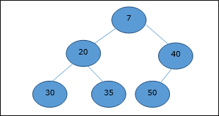
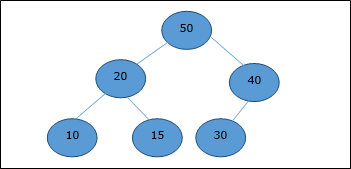
Let us consider the same example discussed previously. Now we want to extract an element. This method will return the root element of the heap.
After deletion of the root element, the last element will be moved to the root position.
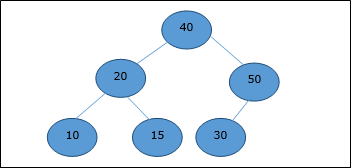
Now, Heapify function will be called. After Heapify, the following heap is generated.
Design and Analysis Bubble Sort
Bubble Sort is an elementary sorting algorithm, which works by repeatedly exchanging adjacent elements, if necessary. When no exchanges are required, the file is sorted.
This is the simplest technique among all sorting algorithms.
Algorithm: Sequential-Bubble-Sort (A) fori← 1 to length [A] do for j ← length [A] down-to i +1 do if A[A] < A[j - 1] then Exchange A[j] ↔ A[j-1]
Implementation
voidbubbleSort(int numbers[], intarray_size) { inti, j, temp; for (i = (array_size - 1); i >= 0; i--) for (j = 1; j <= i; j++) if (numbers[j - 1] > numbers[j]) { temp = numbers[j-1]; numbers[j - 1] = numbers[j]; numbers[j] = temp; } } Analysis
Here, the number of comparisons are
1 + 2 + 3 +...+ (n - 1) = n(n - 1)/2 = O(n 2)
Clearly, the graph shows the n2 nature of the bubble sort.
In this algorithm, the number of comparison is irrespective of the data set, i.e. whether the provided input elements are in sorted order or in reverse order or at random.
Memory Requirement
From the algorithm stated above, it is clear that bubble sort does not require extra memory.
Example
| Unsorted list: |
|
1st iteration:
| 5 > 2 swap |
| |||||||
| 5 > 1 swap |
| |||||||
| 5 > 4 swap |
| |||||||
| 5 > 3 swap |
| |||||||
| 5 < 7 no swap |
| |||||||
| 7 > 6 swap |
|
2nd iteration:
| 2 > 1 swap |
| |||||||
| 2 < 4 no swap |
| |||||||
| 4 > 3 swap |
| |||||||
| 4 < 5 no swap |
| |||||||
| 5 < 6 no swap |
|
There is no change in 3rd, 4th, 5th and 6th iteration.
Finally,
| the sorted list is |
|
Design and Analysis Insertion Sort
Insertion sort is a very simple method to sort numbers in an ascending or descending order. This method follows the incremental method. It can be compared with the technique how cards are sorted at the time of playing a game.
The numbers, which are needed to be sorted, are known as keys. Here is the algorithm of the insertion sort method.
Algorithm: Insertion-Sort(A) for j = 2 to A.length key = A[j] i = j – 1 while i > 0 and A[i] > key A[i + 1] = A[i] i = i -1 A[i + 1] = key
Analysis
Run time of this algorithm is very much dependent on the given input.
If the given numbers are sorted, this algorithm runs in O(n) time. If the given numbers are in reverse order, the algorithm runs in O(n2) time.
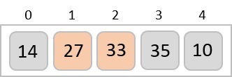
Example
| Unsorted list: |
|
1st iteration:
Key = a[2] = 13
a[1] = 2 < 13
| Swap, no swap |
|
2nd iteration:
Key = a[3] = 5
a[2] = 13 > 5
| Swap 5 and 13 |
|
Next, a[1] = 2 < 13
| Swap, no swap |
|
3rd iteration:
Key = a[4] = 18
a[3] = 13 < 18,
a[2] = 5 < 18,
a[1] = 2 < 18
| Swap, no swap |
|
4th iteration:
Key = a[5] = 14
a[4] = 18 > 14
| Swap 18 and 14 |
|
Next, a[3] = 13 < 14,
a[2] = 5 < 14,
a[1] = 2 < 14
Finally,
| the sorted list is |
|
Design and Analysis Selection Sort
This type of sorting is called Selection Sort as it works by repeatedly sorting elements. It works as follows: first find the smallest in the array and exchange it with the element in the first position, then find the second smallest element and exchange it with the element in the second position, and continue in this way until the entire array is sorted.
Algorithm: Selection-Sort (A) fori ← 1 to n-1 do min j ← i; min x ← A[i] for j ←i + 1 to n do if A[j] < min x then min j ← j min x ← A[j] A[min j] ← A [i] A[i] ← min x
Selection sort is among the simplest of sorting techniques and it works very well for small files. It has a quite important application as each item is actually moved at the most once.
Section sort is a method of choice for sorting files with very large objects (records) and small keys. The worst case occurs if the array is already sorted in a descending order and we want to sort them in an ascending order.
Nonetheless, the time required by selection sort algorithm is not very sensitive to the original order of the array to be sorted: the test if A[j] < min x is executed exactly the same number of times in every case.
Selection sort spends most of its time trying to find the minimum element in the unsorted part of the array. It clearly shows the similarity between Selection sort and Bubble sort.
-
Bubble sort selects the maximum remaining elements at each stage, but wastes some effort imparting some order to an unsorted part of the array.
-
Selection sort is quadratic in both the worst and the average case, and requires no extra memory.
For each i from 1 to n - 1 , there is one exchange and n - i comparisons, so there is a total of n - 1 exchanges and
(n − 1) + (n − 2) + ...+ 2 + 1 = n(n − 1)/2 comparisons.
These observations hold, no matter what the input data is.
In the worst case, this could be quadratic, but in the average case, this quantity is O(n log n) . It implies that the running time of Selection sort is quite insensitive to the input.
Implementation
Void Selection-Sort(int numbers[], int array_size) { int i, j; int min, temp; for (i = 0; I < array_size-1; i++) { min = i; for (j = i+1; j < array_size; j++) if (numbers[j] < numbers[min]) min = j; temp = numbers[i]; numbers[i] = numbers[min]; numbers[min] = temp; } } Example
1st iteration:
Smallest = 5
2 < 5, smallest = 2
1 < 2, smallest = 1
4 > 1, smallest = 1
3 > 1, smallest = 1
2nd iteration:
Smallest = 2
2 < 5, smallest = 2
2 < 4, smallest = 2
2 < 3, smallest = 2
3rd iteration:
Smallest = 5
4 < 5, smallest = 4
3 < 4, smallest = 3
4th iteration:
Smallest = 4
4 < 5, smallest = 4
Finally,
| the sorted list is |
|
Design and Analysis Quick Sort
It is used on the principle of divide-and-conquer. Quick sort is an algorithm of choice in many situations as it is not difficult to implement. It is a good general purpose sort and it consumes relatively fewer resources during execution.
Advantages
-
It is in-place since it uses only a small auxiliary stack.
-
It requires only n (log n) time to sort n items.
-
It has an extremely short inner loop.
-
This algorithm has been subjected to a thorough mathematical analysis, a very precise statement can be made about performance issues.
Disadvantages
-
It is recursive. Especially, if recursion is not available, the implementation is extremely complicated.
-
It requires quadratic (i.e., n2) time in the worst-case.
-
It is fragile, i.e. a simple mistake in the implementation can go unnoticed and cause it to perform badly.
Quick sort works by partitioning a given array A[p ... r] into two non-empty sub array A[p ... q] and A[q+1 ... r] such that every key in A[p ... q] is less than or equal to every key in A[q+1 ... r] .
Then, the two sub-arrays are sorted by recursive calls to Quick sort. The exact position of the partition depends on the given array and index q is computed as a part of the partitioning procedure.
Algorithm: Quick-Sort (A, p, r) if p < r then q Partition (A, p, r) Quick-Sort (A, p, q) Quick-Sort (A, q + r, r)
Note that to sort the entire array, the initial call should be Quick-Sort (A, 1, length[A])
As a first step, Quick Sort chooses one of the items in the array to be sorted as pivot. Then, the array is partitioned on either side of the pivot. Elements that are less than or equal to pivot will move towards the left, while the elements that are greater than or equal to pivot will move towards the right.
Partitioning the Array
Partitioning procedure rearranges the sub-arrays in-place.
Function: Partition (A, p, r) x ← A[p] i ← p-1 j ← r+1 while TRUE do Repeat j ← j - 1 until A[j] ≤ x Repeat i← i+1 until A[i] ≥ x if i < j then exchange A[i] ↔ A[j] else return j
Analysis
The worst case complexity of Quick-Sort algorithm is O(n2) . However using this technique, in average cases generally we get the output in O(n log n) time.
Design and Analysis Radix Sort
Radix sort is a small method that many people intuitively use when alphabetizing a large list of names. Specifically, the list of names is first sorted according to the first letter of each name, that is, the names are arranged in 26 classes.
Intuitively, one might want to sort numbers on their most significant digit. However, Radix sort works counter-intuitively by sorting on the least significant digits first. On the first pass, all the numbers are sorted on the least significant digit and combined in an array. Then on the second pass, the entire numbers are sorted again on the second least significant digits and combined in an array and so on.
Algorithm: Radix-Sort (list, n) shift = 1 for loop = 1 to keysize do for entry = 1 to n do bucketnumber = (list[entry].key / shift) mod 10 append (bucket[bucketnumber], list[entry]) list = combinebuckets() shift = shift * 10
Analysis
Each key is looked at once for each digit (or letter if the keys are alphabetic) of the longest key. Hence, if the longest key has m digits and there are n keys, radix sort has order O(m.n).
However, if we look at these two values, the size of the keys will be relatively small when compared to the number of keys. For example, if we have six-digit keys, we could have a million different records.
Here, we see that the size of the keys is not significant, and this algorithm is of linear complexity O(n).
Example
Following example shows how Radix sort operates on seven 3-digits number.
| Input | 1st Pass | 2nd Pass | 3rd Pass |
|---|---|---|---|
| 329 | 720 | 720 | 329 |
| 457 | 355 | 329 | 355 |
| 657 | 436 | 436 | 436 |
| 839 | 457 | 839 | 457 |
| 436 | 657 | 355 | 657 |
| 720 | 329 | 457 | 720 |
| 355 | 839 | 657 | 839 |
In the above example, the first column is the input. The remaining columns show the list after successive sorts on increasingly significant digits position. The code for Radix sort assumes that each element in an array A of n elements has d digits, where digit 1 is the lowest-order digit and d is the highest-order digit.
Deterministic vs. Nondeterministic Computations
To understand class P and NP, first we should know the computational model. Hence, in this chapter we will discuss two important computational models.
Deterministic Computation and the Class P
Deterministic Turing Machine
One of these models is deterministic one-tape Turing machine. This machine consists of a finite state control, a read-write head and a two-way tape with infinite sequence.
Following is the schematic diagram of a deterministic one-tape Turing machine.
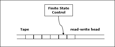
A program for a deterministic Turing machine specifies the following information −
- A finite set of tape symbols (input symbols and a blank symbol)
- A finite set of states
- A transition function
In algorithmic analysis, if a problem is solvable in polynomial time by a deterministic one tape Turing machine, the problem belongs to P class.
Nondeterministic Computation and the Class NP
Nondeterministic Turing Machine
To solve the computational problem, another model is the Non-deterministic Turing Machine (NDTM). The structure of NDTM is similar to DTM, however here we have one additional module known as the guessing module, which is associated with one write-only head.
Following is the schematic diagram.
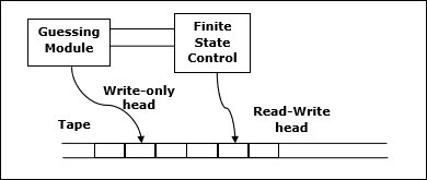
If the problem is solvable in polynomial time by a non-deterministic Turing machine, the problem belongs to NP class.
Design and Analysis Max Cliques
In an undirected graph, a clique is a complete sub-graph of the given graph. Complete sub-graph means, all the vertices of this sub-graph is connected to all other vertices of this sub-graph.
The Max-Clique problem is the computational problem of finding maximum clique of the graph. Max clique is used in many real-world problems.
Let us consider a social networking application, where vertices represent people's profile and the edges represent mutual acquaintance in a graph. In this graph, a clique represents a subset of people who all know each other.
To find a maximum clique, one can systematically inspect all subsets, but this sort of brute-force search is too time-consuming for networks comprising more than a few dozen vertices.
Algorithm: Max-Clique (G, n, k) S := Φ for i = 1 to k do t := choice (1…n) if t Є S then return failure S := S ∪ t for all pairs (i, j) such that i Є S and j Є S and i ≠ j do if (i, j) is not a edge of the graph then return failure return success
Analysis
Max-Clique problem is a non-deterministic algorithm. In this algorithm, first we try to determine a set of k distinct vertices and then we try to test whether these vertices form a complete graph.
There is no polynomial time deterministic algorithm to solve this problem. This problem is NP-Complete.
Example
Take a look at the following graph. Here, the sub-graph containing vertices 2, 3, 4 and 6 forms a complete graph. Hence, this sub-graph is a clique. As this is the maximum complete sub-graph of the provided graph, it's a 4-Clique.
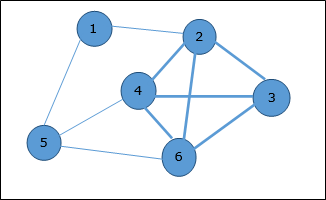
Design and Analysis Vertex Cover
A vertex-cover of an undirected graph G = (V, E) is a subset of vertices V' ⊆ V such that if edge (u, v) is an edge of G , then either u in V or v in V' or both.
Find a vertex-cover of maximum size in a given undirected graph. This optimal vertexcover is the optimization version of an NP-complete problem. However, it is not too hard to find a vertex-cover that is near optimal.
APPROX-VERTEX_COVER (G: Graph) c ← { } E' ← E[G] while E' is not empty do Let (u, v) be an arbitrary edge of E' c ← c U {u, v} Remove from E' every edge incident on either u or v return c Example
The set of edges of the given graph is −
{(1,6),(1,2),(1,4),(2,3),(2,4),(6,7),(4,7),(7,8),(3,8),(3,5),(8,5)}
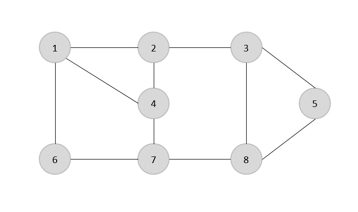
Now, we start by selecting an arbitrary edge (1,6). We eliminate all the edges, which are either incident to vertex 1 or 6 and we add edge (1,6) to cover.
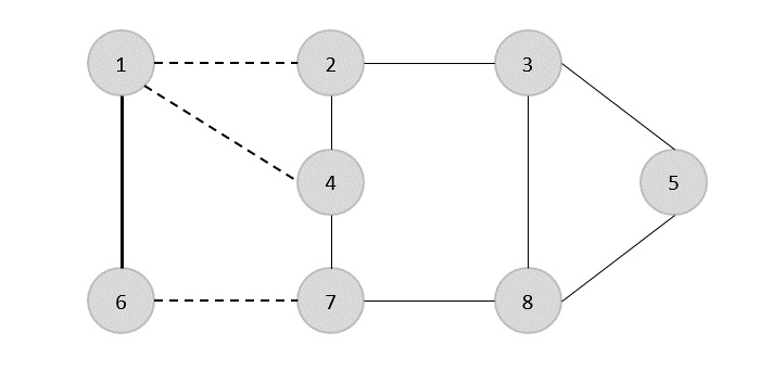
In the next step, we have chosen another edge (2,3) at random
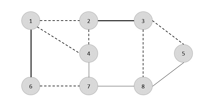
Now we select another edge (4,7).
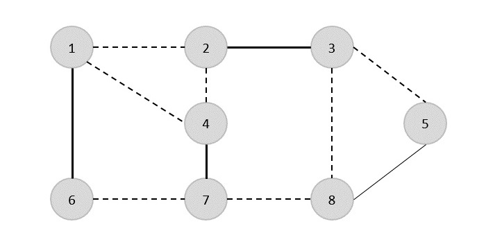
We select another edge (8,5).
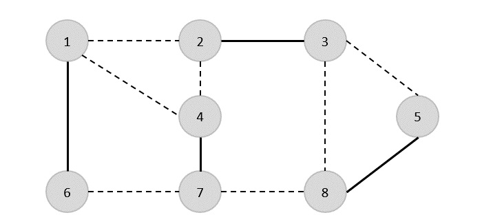
Hence, the vertex cover of this graph is {1,2,4,5}.
Analysis
It is easy to see that the running time of this algorithm is O(V + E) , using adjacency list to represent E' .
Design and Analysis P and NP Class
In Computer Science, many problems are solved where the objective is to maximize or minimize some values, whereas in other problems we try to find whether there is a solution or not. Hence, the problems can be categorized as follows −
Optimization Problem
Optimization problems are those for which the objective is to maximize or minimize some values. For example,
-
Finding the minimum number of colors needed to color a given graph.
-
Finding the shortest path between two vertices in a graph.
Decision Problem
There are many problems for which the answer is a Yes or a No. These types of problems are known as decision problems. For example,
-
Whether a given graph can be colored by only 4-colors.
-
Finding Hamiltonian cycle in a graph is not a decision problem, whereas checking a graph is Hamiltonian or not is a decision problem.
What is Language?
Every decision problem can have only two answers, yes or no. Hence, a decision problem may belong to a language if it provides an answer 'yes' for a specific input. A language is the totality of inputs for which the answer is Yes. Most of the algorithms discussed in the previous chapters are polynomial time algorithms.
For input size n , if worst-case time complexity of an algorithm is O(nk) , where k is a constant, the algorithm is a polynomial time algorithm.
Algorithms such as Matrix Chain Multiplication, Single Source Shortest Path, All Pair Shortest Path, Minimum Spanning Tree, etc. run in polynomial time. However there are many problems, such as traveling salesperson, optimal graph coloring, Hamiltonian cycles, finding the longest path in a graph, and satisfying a Boolean formula, for which no polynomial time algorithms is known. These problems belong to an interesting class of problems, called the NP-Complete problems, whose status is unknown.
In this context, we can categorize the problems as follows −
P-Class
The class P consists of those problems that are solvable in polynomial time, i.e. these problems can be solved in time O(nk) in worst-case, where k is constant.
These problems are called tractable, while others are called intractable or superpolynomial.
Formally, an algorithm is polynomial time algorithm, if there exists a polynomial p(n) such that the algorithm can solve any instance of size n in a time O(p(n)) .
Problem requiring Ω(n50) time to solve are essentially intractable for large n . Most known polynomial time algorithm run in time O(nk) for fairly low value of k .
The advantages in considering the class of polynomial-time algorithms is that all reasonable deterministic single processor model of computation can be simulated on each other with at most a polynomial slow-d
NP-Class
The class NP consists of those problems that are verifiable in polynomial time. NP is the class of decision problems for which it is easy to check the correctness of a claimed answer, with the aid of a little extra information. Hence, we aren't asking for a way to find a solution, but only to verify that an alleged solution really is correct.
Every problem in this class can be solved in exponential time using exhaustive search.
P versus NP
Every decision problem that is solvable by a deterministic polynomial time algorithm is also solvable by a polynomial time non-deterministic algorithm.
All problems in P can be solved with polynomial time algorithms, whereas all problems in NP - P are intractable.
It is not known whether P = NP . However, many problems are known in NP with the property that if they belong to P, then it can be proved that P = NP.
If P ≠ NP , there are problems in NP that are neither in P nor in NP-Complete.
The problem belongs to class P if it's easy to find a solution for the problem. The problem belongs to NP, if it's easy to check a solution that may have been very tedious to find.
Design and Analysis Cook's Theorem
Stephen Cook presented four theorems in his paper "The Complexity of Theorem Proving Procedures". These theorems are stated below. We do understand that many unknown terms are being used in this chapter, but we don't have any scope to discuss everything in detail.
Following are the four theorems by Stephen Cook −
Theorem-1
If a set S of strings is accepted by some non-deterministic Turing machine within polynomial time, then S is P-reducible to {DNF tautologies}.
Theorem-2
The following sets are P-reducible to each other in pairs (and hence each has the same polynomial degree of difficulty): {tautologies}, {DNF tautologies}, D3, {sub-graph pairs}.
Theorem-3
-
For any TQ(k) of type Q, $\mathbf{\frac{T_{Q}(k)}{\frac{\sqrt{k}}{(log\:k)^2}}}$ is unbounded
-
There is a TQ(k) of type Q such that $T_{Q}(k)\leqslant 2^{k(log\:k)^2}$
Theorem-4
If the set S of strings is accepted by a non-deterministic machine within time T(n) = 2n , and if TQ(k) is an honest (i.e. real-time countable) function of type Q, then there is a constant K, so S can be recognized by a deterministic machine within time TQ(K8n) .
-
First, he emphasized the significance of polynomial time reducibility. It means that if we have a polynomial time reduction from one problem to another, this ensures that any polynomial time algorithm from the second problem can be converted into a corresponding polynomial time algorithm for the first problem.
-
Second, he focused attention on the class NP of decision problems that can be solved in polynomial time by a non-deterministic computer. Most of the intractable problems belong to this class, NP.
-
Third, he proved that one particular problem in NP has the property that every other problem in NP can be polynomially reduced to it. If the satisfiability problem can be solved with a polynomial time algorithm, then every problem in NP can also be solved in polynomial time. If any problem in NP is intractable, then satisfiability problem must be intractable. Thus, satisfiability problem is the hardest problem in NP.
-
Fourth, Cook suggested that other problems in NP might share with the satisfiability problem this property of being the hardest member of NP.
NP Hard and NP-Complete Classes
A problem is in the class NPC if it is in NP and is as hard as any problem in NP. A problem is NP-hard if all problems in NP are polynomial time reducible to it, even though it may not be in NP itself.
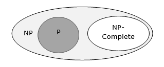
If a polynomial time algorithm exists for any of these problems, all problems in NP would be polynomial time solvable. These problems are called NP-complete. The phenomenon of NP-completeness is important for both theoretical and practical reasons.
Definition of NP-Completeness
A language B is NP-complete if it satisfies two conditions
-
B is in NP
-
Every A in NP is polynomial time reducible to B.
If a language satisfies the second property, but not necessarily the first one, the language B is known as NP-Hard. Informally, a search problem B is NP-Hard if there exists some NP-Complete problem A that Turing reduces to B.
The problem in NP-Hard cannot be solved in polynomial time, until P = NP. If a problem is proved to be NPC, there is no need to waste time on trying to find an efficient algorithm for it. Instead, we can focus on design approximation algorithm.
NP-Complete Problems
Following are some NP-Complete problems, for which no polynomial time algorithm is known.
- Determining whether a graph has a Hamiltonian cycle
- Determining whether a Boolean formula is satisfiable, etc.
NP-Hard Problems
The following problems are NP-Hard
- The circuit-satisfiability problem
- Set Cover
- Vertex Cover
- Travelling Salesman Problem
In this context, now we will discuss TSP is NP-Complete
TSP is NP-Complete
The traveling salesman problem consists of a salesman and a set of cities. The salesman has to visit each one of the cities starting from a certain one and returning to the same city. The challenge of the problem is that the traveling salesman wants to minimize the total length of the trip
Proof
To prove TSP is NP-Complete , first we have to prove that TSP belongs to NP . In TSP, we find a tour and check that the tour contains each vertex once. Then the total cost of the edges of the tour is calculated. Finally, we check if the cost is minimum. This can be completed in polynomial time. Thus TSP belongs to NP .
Secondly, we have to prove that TSP is NP-hard . To prove this, one way is to show that Hamiltonian cycle ≤p TSP (as we know that the Hamiltonian cycle problem is NPcomplete).
Assume G = (V, E) to be an instance of Hamiltonian cycle.
Hence, an instance of TSP is constructed. We create the complete graph G' = (V, E') , where
$$E^{'}=\lbrace(i, j)\colon i, j \in V \:\:and\:i\neq j$$
Thus, the cost function is defined as follows −
$$t(i,j)=\begin{cases}0 & if\: (i, j)\: \in E\\1 & otherwise\end{cases}$$
Now, suppose that a Hamiltonian cycle h exists in G . It is clear that the cost of each edge in h is 0 in G' as each edge belongs to E . Therefore, h has a cost of 0 in G' . Thus, if graph G has a Hamiltonian cycle, then graph G' has a tour of 0 cost.
Conversely, we assume that G' has a tour h' of cost at most 0. The cost of edges in E' are 0 and 1 by definition. Hence, each edge must have a cost of 0 as the cost of h' is 0. We therefore conclude that h' contains only edges in E .
We have thus proven that G has a Hamiltonian cycle, if and only if G' has a tour of cost at most 0. TSP is NP-complete.
Design and Analysis Hill Climbing Algorithm
The algorithms discussed in the previous chapters run systematically. To achieve the goal, one or more previously explored paths toward the solution need to be stored to find the optimal solution.
For many problems, the path to the goal is irrelevant. For example, in N-Queens problem, we don't need to care about the final configuration of the queens as well as in which order the queens are added.
Hill Climbing
Hill Climbing is a technique to solve certain optimization problems. In this technique, we start with a sub-optimal solution and the solution is improved repeatedly until some condition is maximized.
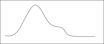
The idea of starting with a sub-optimal solution is compared to starting from the base of the hill, improving the solution is compared to walking up the hill, and finally maximizing some condition is compared to reaching the top of the hill.
Hence, the hill climbing technique can be considered as the following phases −
- Constructing a sub-optimal solution obeying the constraints of the problem
- Improving the solution step-by-step
- Improving the solution until no more improvement is possible
Hill Climbing technique is mainly used for solving computationally hard problems. It looks only at the current state and immediate future state. Hence, this technique is memory efficient as it does not maintain a search tree.
Algorithm: Hill Climbing Evaluate the initial state. Loop until a solution is found or there are no new operators left to be applied: - Select and apply a new operator - Evaluate the new state: goal -→ quit better than current state -→ new current state
Iterative Improvement
In iterative improvement method, the optimal solution is achieved by making progress towards an optimal solution in every iteration. However, this technique may encounter local maxima. In this situation, there is no nearby state for a better solution.
This problem can be avoided by different methods. One of these methods is simulated annealing.
Random Restart
This is another method of solving the problem of local optima. This technique conducts a series of searches. Every time, it starts from a randomly generated initial state. Hence, optima or nearly optimal solution can be obtained comparing the solutions of searches performed.
Problems of Hill Climbing Technique
Local Maxima
If the heuristic is not convex, Hill Climbing may converge to local maxima, instead of global maxima.
Ridges and Alleys
If the target function creates a narrow ridge, then the climber can only ascend the ridge or descend the alley by zig-zagging. In this scenario, the climber needs to take very small steps requiring more time to reach the goal.
Plateau
A plateau is encountered when the search space is flat or sufficiently flat that the value returned by the target function is indistinguishable from the value returned for nearby regions, due to the precision used by the machine to represent its value.
Complexity of Hill Climbing Technique
This technique does not suffer from space related issues, as it looks only at the current state. Previously explored paths are not stored.
For most of the problems in Random-restart Hill Climbing technique, an optimal solution can be achieved in polynomial time. However, for NP-Complete problems, computational time can be exponential based on the number of local maxima.
Applications of Hill Climbing Technique
Hill Climbing technique can be used to solve many problems, where the current state allows for an accurate evaluation function, such as Network-Flow, Travelling Salesman problem, 8-Queens problem, Integrated Circuit design, etc.
Hill Climbing is used in inductive learning methods too. This technique is used in robotics for coordination among multiple robots in a team. There are many other problems where this technique is used.
Example
This technique can be applied to solve the travelling salesman problem. First an initial solution is determined that visits all the cities exactly once. Hence, this initial solution is not optimal in most of the cases. Even this solution can be very poor. The Hill Climbing algorithm starts with such an initial solution and makes improvements to it in an iterative way. Eventually, a much shorter route is likely to be obtained.
Useful Video Courses

Video

Video

Video

Video

Video

Video
Design and Analysis of Algorithms Lab Manual Using Java
Source: https://www.tutorialspoint.com/design_and_analysis_of_algorithms/design_and_analysis_of_algorithms_quick_guide.htm
0 Response to "Design and Analysis of Algorithms Lab Manual Using Java"
Post a Comment